向量量化範例

此範例展示如何使用 KBinsDiscretizer 對一組玩具影像（浣熊臉）執行向量量化。

# Authors: The scikit-learn developers
# SPDX-License-Identifier: BSD-3-Clause

原始影像

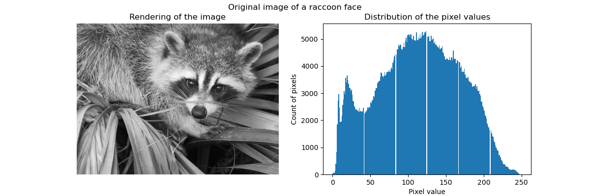
我們首先從 SciPy 載入浣熊臉部影像。我們還將檢查一些關於影像的資訊，例如影像的形狀和用於儲存影像的資料類型。

請注意，根據 SciPy 版本，我們必須調整匯入，因為傳回影像的函數不在同一個模組中。此外，SciPy >= 1.10 需要安裝 pooch 套件。

try:  # Scipy >= 1.10
    from scipy.datasets import face
except ImportError:
    from scipy.misc import face

raccoon_face = face(gray=True)

print(f"The dimension of the image is {raccoon_face.shape}")
print(f"The data used to encode the image is of type {raccoon_face.dtype}")
print(f"The number of bytes taken in RAM is {raccoon_face.nbytes}")

The dimension of the image is (768, 1024)
The data used to encode the image is of type uint8
The number of bytes taken in RAM is 786432

因此，影像是一個 2D 陣列，高度為 768 像素，寬度為 1024 像素。每個值都是一個 8 位元無號整數，這表示影像使用每個像素 8 位元進行編碼。影像的總記憶體使用量為 786 KB（1 個位元組等於 8 位元）。

使用 8 位元無號整數表示影像最多使用 256 種不同的灰階陰影進行編碼。我們可以檢查這些值的分布。

import matplotlib.pyplot as plt

fig, ax = plt.subplots(ncols=2, figsize=(12, 4))

ax[0].imshow(raccoon_face, cmap=plt.cm.gray)
ax[0].axis("off")
ax[0].set_title("Rendering of the image")
ax[1].hist(raccoon_face.ravel(), bins=256)
ax[1].set_xlabel("Pixel value")
ax[1].set_ylabel("Count of pixels")
ax[1].set_title("Distribution of the pixel values")
_ = fig.suptitle("Original image of a raccoon face")

透過向量量化壓縮

透過向量量化進行壓縮背後的概念是減少用於表示影像的灰階數量。例如，我們可以使用 8 個值而不是 256 個值。因此，這表示我們可以有效率地使用 3 位元而不是 8 位元來編碼單個像素，因此將記憶體使用量減少大約 2.5 倍。我們稍後將討論這個記憶體使用量。

編碼策略

可以使用 KBinsDiscretizer 完成壓縮。我們需要選擇一種策略來定義要次取樣的 8 個灰階值。最簡單的策略是定義它們等間隔，這相當於設定 strategy="uniform"。從先前的長條圖中，我們知道這種策略肯定不是最佳的。

from sklearn.preprocessing import KBinsDiscretizer

n_bins = 8
encoder = KBinsDiscretizer(
    n_bins=n_bins,
    encode="ordinal",
    strategy="uniform",
    random_state=0,
)
compressed_raccoon_uniform = encoder.fit_transform(raccoon_face.reshape(-1, 1)).reshape(
    raccoon_face.shape
)

fig, ax = plt.subplots(ncols=2, figsize=(12, 4))
ax[0].imshow(compressed_raccoon_uniform, cmap=plt.cm.gray)
ax[0].axis("off")
ax[0].set_title("Rendering of the image")
ax[1].hist(compressed_raccoon_uniform.ravel(), bins=256)
ax[1].set_xlabel("Pixel value")
ax[1].set_ylabel("Count of pixels")
ax[1].set_title("Sub-sampled distribution of the pixel values")
_ = fig.suptitle("Raccoon face compressed using 3 bits and a uniform strategy")

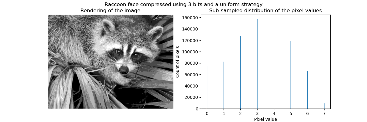
在質量上，我們可以發現一些小區域，我們可以在其中看到壓縮的效果（例如，右下角的葉子）。但畢竟，結果影像仍然看起來不錯。

我們觀察到像素值的分布已映射到 8 個不同的值。我們可以檢查這些值與原始像素值之間的對應關係。

bin_edges = encoder.bin_edges_[0]
bin_center = bin_edges[:-1] + (bin_edges[1:] - bin_edges[:-1]) / 2
bin_center

array([ 15.625,  46.875,  78.125, 109.375, 140.625, 171.875, 203.125,
       234.375])

_, ax = plt.subplots()
ax.hist(raccoon_face.ravel(), bins=256)
color = "tab:orange"
for center in bin_center:
    ax.axvline(center, color=color)
    ax.text(center - 10, ax.get_ybound()[1] + 100, f"{center:.1f}", color=color)

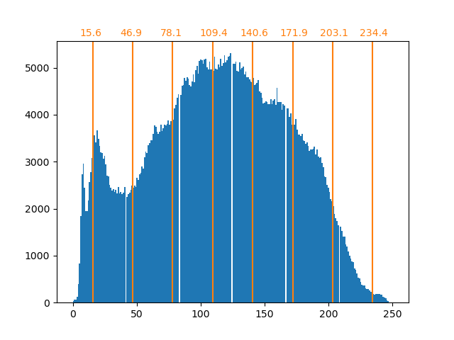
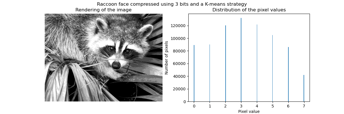
如先前所述，均勻取樣策略不是最佳的。例如，請注意，映射到值 7 的像素將編碼相當少量的資訊，而映射的值 3 將表示大量的計數。我們可以改為使用聚類策略（例如 k 平均值）來尋找更佳的映射。

encoder = KBinsDiscretizer(
    n_bins=n_bins,
    encode="ordinal",
    strategy="kmeans",
    random_state=0,
)
compressed_raccoon_kmeans = encoder.fit_transform(raccoon_face.reshape(-1, 1)).reshape(
    raccoon_face.shape
)

fig, ax = plt.subplots(ncols=2, figsize=(12, 4))
ax[0].imshow(compressed_raccoon_kmeans, cmap=plt.cm.gray)
ax[0].axis("off")
ax[0].set_title("Rendering of the image")
ax[1].hist(compressed_raccoon_kmeans.ravel(), bins=256)
ax[1].set_xlabel("Pixel value")
ax[1].set_ylabel("Number of pixels")
ax[1].set_title("Distribution of the pixel values")
_ = fig.suptitle("Raccoon face compressed using 3 bits and a K-means strategy")

bin_edges = encoder.bin_edges_[0]
bin_center = bin_edges[:-1] + (bin_edges[1:] - bin_edges[:-1]) / 2
bin_center

array([ 18.90885631,  53.34346583,  82.64447187, 109.28225276,
       134.70763101, 159.78681467, 185.17226834, 224.02069427])

_, ax = plt.subplots()
ax.hist(raccoon_face.ravel(), bins=256)
color = "tab:orange"
for center in bin_center:
    ax.axvline(center, color=color)
    ax.text(center - 10, ax.get_ybound()[1] + 100, f"{center:.1f}", color=color)

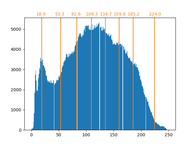
現在，箱中的計數更加平衡，並且它們的中心不再等間隔。請注意，我們可以透過使用 strategy="quantile" 而不是 strategy="kmeans" 來強制每個箱中有相同數量的像素。

記憶體佔用

我們之前說過，我們應該節省 8 倍的記憶體。讓我們驗證一下。

print(f"The number of bytes taken in RAM is {compressed_raccoon_kmeans.nbytes}")
print(f"Compression ratio: {compressed_raccoon_kmeans.nbytes / raccoon_face.nbytes}")

The number of bytes taken in RAM is 6291456
Compression ratio: 8.0

令人驚訝的是，我們發現壓縮後的影像比原始影像佔用了 x8 倍的記憶體。這確實與我們預期的相反。原因主要在於用於編碼影像的資料類型。

print(f"Type of the compressed image: {compressed_raccoon_kmeans.dtype}")

Type of the compressed image: float64

事實上，KBinsDiscretizer 的輸出是一個 64 位元浮點數陣列。這表示它佔用了 x8 倍的記憶體。但是，我們使用此 64 位元浮點數表示來編碼 8 個值。事實上，只有在我們將壓縮後的影像轉換為 3 位元整數陣列時，才能節省記憶體。我們可以使用方法 numpy.ndarray.astype。但是，不存在 3 位元整數表示，並且為了編碼這 8 個值，我們也需要使用 8 位元無號整數表示。

實際上，觀察記憶體增益需要原始影像採用 64 位元浮點數表示。

相關範例

使用字典學習進行影像降噪

使用字典學習進行影像降噪

辨識手寫數字

辨識手寫數字

在硬幣影像上進行結構化 Ward 階層式群集的示範

在硬幣影像上進行結構化 Ward 階層式群集的示範

將希臘硬幣圖片分割成區域

將希臘硬幣圖片分割成區域