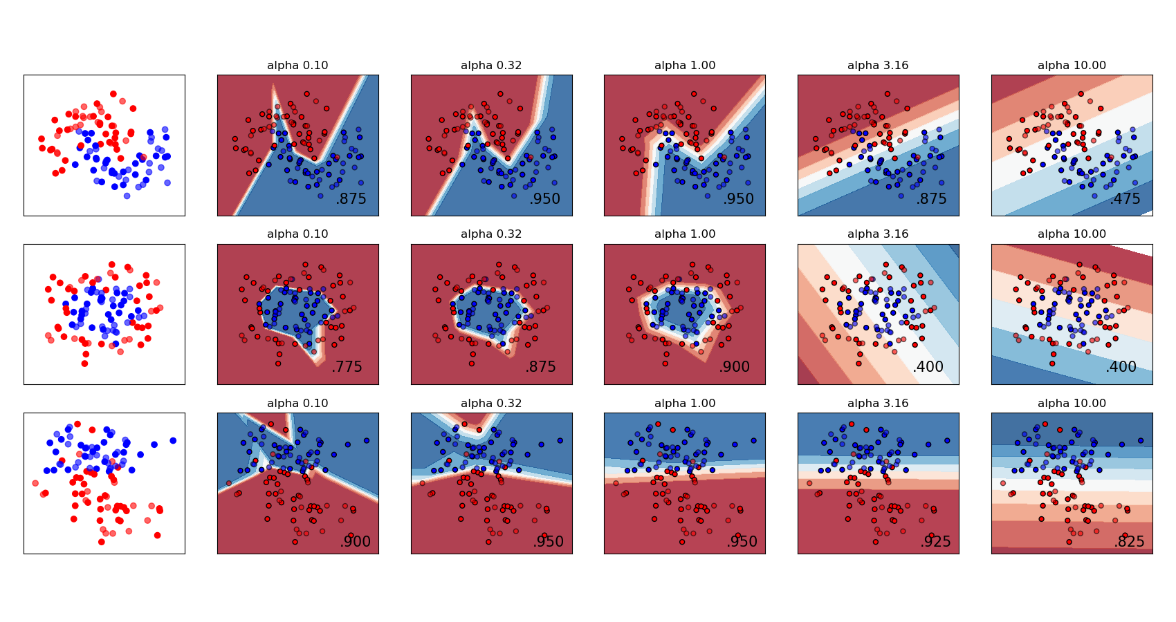
多層感知器中變化的正規化#

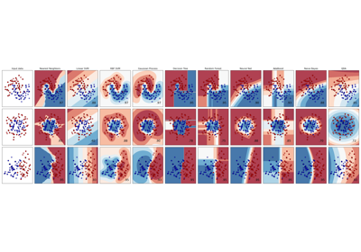
合成資料集上正規化參數 'alpha' 的不同值的比較。此圖顯示不同的 alpha 值會產生不同的決策函數。

Alpha 是正規化項（又稱懲罰項）的參數，透過限制權重的大小來對抗過擬合。增加 alpha 可以透過鼓勵較小的權重來修正高變異數（過擬合的徵兆），從而產生曲率較小的決策邊界圖。同樣地，減少 alpha 可以透過鼓勵較大的權重來修正高偏差（欠擬合的徵兆），可能導致更複雜的決策邊界。

alpha 0.10, alpha 0.32, alpha 1.00, alpha 3.16, alpha 10.00, alpha 0.10, alpha 0.32, alpha 1.00, alpha 3.16, alpha 10.00, alpha 0.10, alpha 0.32, alpha 1.00, alpha 3.16, alpha 10.00

# Authors: The scikit-learn developers
# SPDX-License-Identifier: BSD-3-Clause

import numpy as np
from matplotlib import pyplot as plt
from matplotlib.colors import ListedColormap

from sklearn.datasets import make_circles, make_classification, make_moons
from sklearn.model_selection import train_test_split
from sklearn.neural_network import MLPClassifier
from sklearn.pipeline import make_pipeline
from sklearn.preprocessing import StandardScaler

h = 0.02  # step size in the mesh

alphas = np.logspace(-1, 1, 5)

classifiers = []
names = []
for alpha in alphas:
    classifiers.append(
        make_pipeline(
            StandardScaler(),
            MLPClassifier(
                solver="lbfgs",
                alpha=alpha,
                random_state=1,
                max_iter=2000,
                early_stopping=True,
                hidden_layer_sizes=[10, 10],
            ),
        )
    )
    names.append(f"alpha {alpha:.2f}")

X, y = make_classification(
    n_features=2, n_redundant=0, n_informative=2, random_state=0, n_clusters_per_class=1
)
rng = np.random.RandomState(2)
X += 2 * rng.uniform(size=X.shape)
linearly_separable = (X, y)

datasets = [
    make_moons(noise=0.3, random_state=0),
    make_circles(noise=0.2, factor=0.5, random_state=1),
    linearly_separable,
]

figure = plt.figure(figsize=(17, 9))
i = 1
# iterate over datasets
for X, y in datasets:
    # split into training and test part
    X_train, X_test, y_train, y_test = train_test_split(
        X, y, test_size=0.4, random_state=42
    )

    x_min, x_max = X[:, 0].min() - 0.5, X[:, 0].max() + 0.5
    y_min, y_max = X[:, 1].min() - 0.5, X[:, 1].max() + 0.5
    xx, yy = np.meshgrid(np.arange(x_min, x_max, h), np.arange(y_min, y_max, h))

    # just plot the dataset first
    cm = plt.cm.RdBu
    cm_bright = ListedColormap(["#FF0000", "#0000FF"])
    ax = plt.subplot(len(datasets), len(classifiers) + 1, i)
    # Plot the training points
    ax.scatter(X_train[:, 0], X_train[:, 1], c=y_train, cmap=cm_bright)
    # and testing points
    ax.scatter(X_test[:, 0], X_test[:, 1], c=y_test, cmap=cm_bright, alpha=0.6)
    ax.set_xlim(xx.min(), xx.max())
    ax.set_ylim(yy.min(), yy.max())
    ax.set_xticks(())
    ax.set_yticks(())
    i += 1

    # iterate over classifiers
    for name, clf in zip(names, classifiers):
        ax = plt.subplot(len(datasets), len(classifiers) + 1, i)
        clf.fit(X_train, y_train)
        score = clf.score(X_test, y_test)

        # Plot the decision boundary. For that, we will assign a color to each
        # point in the mesh [x_min, x_max] x [y_min, y_max].
        if hasattr(clf, "decision_function"):
            Z = clf.decision_function(np.column_stack([xx.ravel(), yy.ravel()]))
        else:
            Z = clf.predict_proba(np.column_stack([xx.ravel(), yy.ravel()]))[:, 1]

        # Put the result into a color plot
        Z = Z.reshape(xx.shape)
        ax.contourf(xx, yy, Z, cmap=cm, alpha=0.8)

        # Plot also the training points
        ax.scatter(
            X_train[:, 0],
            X_train[:, 1],
            c=y_train,
            cmap=cm_bright,
            edgecolors="black",
            s=25,
        )
        # and testing points
        ax.scatter(
            X_test[:, 0],
            X_test[:, 1],
            c=y_test,
            cmap=cm_bright,
            alpha=0.6,
            edgecolors="black",
            s=25,
        )

        ax.set_xlim(xx.min(), xx.max())
        ax.set_ylim(yy.min(), yy.max())
        ax.set_xticks(())
        ax.set_yticks(())
        ax.set_title(name)
        ax.text(
            xx.max() - 0.3,
            yy.min() + 0.3,
            f"{score:.3f}".lstrip("0"),
            size=15,
            horizontalalignment="right",
        )
        i += 1

figure.subplots_adjust(left=0.02, right=0.98)
plt.show()