注意
前往結尾下載完整的範例程式碼。或者透過 JupyterLite 或 Binder 在您的瀏覽器中執行此範例
使用不同的 SVM 核心繪製分類邊界#
此範例展示 SVC(支持向量分類器)中不同的核心如何影響二維二元分類問題中的分類邊界。
SVC 旨在透過最大化每個類別最外層資料點之間的邊界,找到有效分離訓練資料中類別的超平面。這是透過找到最佳權重向量 \(w\) 來實現,該向量定義決策邊界超平面,並最小化誤分類樣本的鉸鏈損失總和,如 hinge_loss 函數所測量。依預設,正規化會套用參數 C=1,其允許一定程度的誤分類容忍度。
如果資料在原始特徵空間中不是線性可分的,則可以設定非線性核心參數。根據核心的不同,此過程會涉及新增新特徵或轉換現有特徵,以豐富資料並可能新增資料意義。當設定不是 "linear" 的核心時,SVC 會套用 核心技巧,此技巧使用核心函數計算成對資料點之間的相似性,而無需明確轉換整個資料集。核心技巧僅考慮所有成對資料點之間的關係,因此勝過否則必要的整個資料集的矩陣轉換。核心函數會使用點積將兩個向量(每對觀測值)對應到其相似性。
然後可以使用核心函數計算超平面,就像資料集以高維空間表示一樣。使用核心函數而不是明確的矩陣轉換可以提高效能,因為核心函數的時間複雜度為 \(O({n}^2)\),而矩陣轉換則根據所套用的特定轉換進行縮放。
在此範例中,我們比較支持向量機最常見的核心類型:線性核心 ("linear")、多項式核心 ("poly")、徑向基底函數核心 ("rbf") 和 S 型核心 ("sigmoid")。
# Authors: The scikit-learn developers
# SPDX-License-Identifier: BSD-3-Clause
建立資料集#
我們建立一個具有 16 個樣本和兩個類別的二維分類資料集。我們繪製樣本,顏色與其各自的目標匹配。
import matplotlib.pyplot as plt
import numpy as np

X = np.array(
    [
        [0.4, -0.7],
        [-1.5, -1.0],
        [-1.4, -0.9],
        [-1.3, -1.2],
        [-1.1, -0.2],
        [-1.2, -0.4],
        [-0.5, 1.2],
        [-1.5, 2.1],
        [1.0, 1.0],
        [1.3, 0.8],
        [1.2, 0.5],
        [0.2, -2.0],
        [0.5, -2.4],
        [0.2, -2.3],
        [0.0, -2.7],
        [1.3, 2.1],
    ]
)

y = np.array([0, 0, 0, 0, 0, 0, 0, 0, 1, 1, 1, 1, 1, 1, 1, 1])

# Plotting settings
fig, ax = plt.subplots(figsize=(4, 3))
x_min, x_max, y_min, y_max = -3, 3, -3, 3
ax.set(xlim=(x_min, x_max), ylim=(y_min, y_max))

# Plot samples by color and add legend
scatter = ax.scatter(X[:, 0], X[:, 1], s=150, c=y, label=y, edgecolors="k")
ax.legend(*scatter.legend_elements(), loc="upper right", title="Classes")
ax.set_title("Samples in two-dimensional feature space")
_ = plt.show()
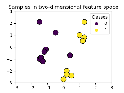
我們可以看到,樣本無法用直線清楚地分隔。
訓練 SVC 模型並繪製決策邊界#
我們定義一個函數,其擬合 SVC 分類器,允許將 kernel 參數作為輸入,然後使用 DecisionBoundaryDisplay 繪製模型學習的決策邊界。
請注意,為了簡單起見,在此範例中,C 參數設定為其預設值 (C=1),並且所有核心的 gamma 參數都設定為 gamma=2,儘管線性核心會自動忽略它。在效能至關重要的真實分類任務中,強烈建議進行參數調整(例如,使用 GridSearchCV)來擷取資料中不同的結構。
在 DecisionBoundaryDisplay 中設定 response_method="predict" 會根據其預測的類別著色區域。使用 response_method="decision_function" 可讓我們也繪製決策邊界及其兩側的邊界。最後,在訓練期間使用的支持向量(始終位於邊界上)透過訓練的 SVC 的 support_vectors_ 屬性來識別,並且也繪製出來。
from sklearn import svm
from sklearn.inspection import DecisionBoundaryDisplay


def plot_training_data_with_decision_boundary(
    kernel, ax=None, long_title=True, support_vectors=True
):
    # Train the SVC
    clf = svm.SVC(kernel=kernel, gamma=2).fit(X, y)

    # Settings for plotting
    if ax is None:
        _, ax = plt.subplots(figsize=(4, 3))
    x_min, x_max, y_min, y_max = -3, 3, -3, 3
    ax.set(xlim=(x_min, x_max), ylim=(y_min, y_max))

    # Plot decision boundary and margins
    common_params = {"estimator": clf, "X": X, "ax": ax}
    DecisionBoundaryDisplay.from_estimator(
        **common_params,
        response_method="predict",
        plot_method="pcolormesh",
        alpha=0.3,
    )
    DecisionBoundaryDisplay.from_estimator(
        **common_params,
        response_method="decision_function",
        plot_method="contour",
        levels=[-1, 0, 1],
        colors=["k", "k", "k"],
        linestyles=["--", "-", "--"],
    )

    if support_vectors:
        # Plot bigger circles around samples that serve as support vectors
        ax.scatter(
            clf.support_vectors_[:, 0],
            clf.support_vectors_[:, 1],
            s=150,
            facecolors="none",
            edgecolors="k",
        )

    # Plot samples by color and add legend
    ax.scatter(X[:, 0], X[:, 1], c=y, s=30, edgecolors="k")
    ax.legend(*scatter.legend_elements(), loc="upper right", title="Classes")
    if long_title:
        ax.set_title(f" Decision boundaries of {kernel} kernel in SVC")
    else:
        ax.set_title(kernel)

    if ax is None:
        plt.show()
線性核心#
線性核心是輸入樣本的點積
然後將其套用到資料集中兩個資料點(樣本)的任意組合。兩個點的點積會決定兩個點之間的 cosine_similarity。值越高,點越相似。
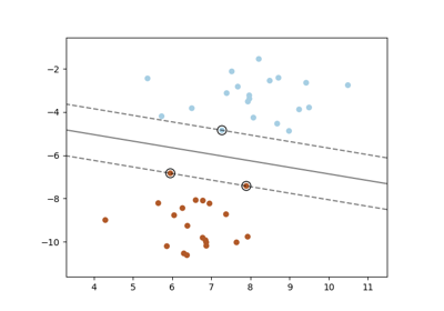
plot_training_data_with_decision_boundary("linear")
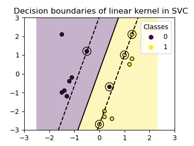
在線性核心上訓練 SVC 會產生未轉換的特徵空間,其中超平面和邊界是直線。由於線性核心缺乏表現力,因此訓練的類別無法完美擷取訓練資料。
多項式核心#
多項式核心會改變相似性的概念。核心函數定義為
其中 \({d}\) 是多項式的次數(degree),\({\gamma}\)(gamma)控制每個個別訓練樣本對決策邊界的影響,而 \({r}\) 是偏差項(coef0),可以將資料向上或向下平移。在這裡,我們使用核心函數中多項式次數的預設值(degree=3)。當 coef0=0(預設值)時,資料只會被轉換,不會加入額外的維度。使用多項式核心等同於先建立 PolynomialFeatures,然後在轉換後的資料上擬合一個具有線性核心的 SVC,儘管對於大多數資料集來說,這種替代方法在計算上會很昂貴。
plot_training_data_with_decision_boundary("poly")
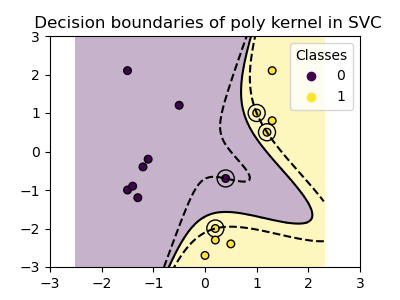
具有 gamma=2 的多項式核心能很好地適應訓練資料,使得超平面兩側的邊界相應彎曲。
RBF 核心#
徑向基函數(RBF)核心,也稱為高斯核心,是 scikit-learn 中支援向量機的預設核心。它測量無限維度中兩個資料點之間的相似性,然後透過多數投票來進行分類。核心函數定義為
其中 \({\gamma}\)(gamma)控制每個個別訓練樣本對決策邊界的影響。
兩個點之間的歐幾里得距離 \(\|\mathbf{x}_1 - \mathbf{x}_2\|^2\) 越大,核心函數的值越接近零。這表示相距較遠的兩個點更可能不相似。
plot_training_data_with_decision_boundary("rbf")
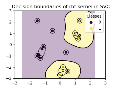
在圖中,我們可以觀察到決策邊界如何傾向於收縮到彼此靠近的資料點周圍。
Sigmoid 核心#
Sigmoid 核心函數定義為
其中核心係數 \({\gamma}\)(gamma)控制每個個別訓練樣本對決策邊界的影響,而 \({r}\) 是偏差項(coef0),可以將資料向上或向下平移。
在 Sigmoid 核心中,兩個資料點之間的相似性是使用雙曲正切函數 (\(\tanh\)) 計算的。核心函數會縮放並可能平移兩個點的點積(\(\mathbf{x}_1\) 和 \(\mathbf{x}_2\))。
plot_training_data_with_decision_boundary("sigmoid")
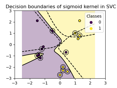
我們可以觀察到,使用 Sigmoid 核心獲得的決策邊界呈現彎曲且不規則的形狀。決策邊界嘗試透過擬合 Sigmoid 形狀的曲線來分離類別,從而產生複雜的邊界,可能無法很好地推廣到未見過的資料。從這個例子可以明顯看出,Sigmoid 核心在處理呈現 Sigmoid 形狀的資料時,具有非常特定的使用案例。在這個例子中,仔細的微調可能會找到更具泛化能力的決策邊界。由於其特殊性,與其他核心相比,Sigmoid 核心在實務中較少使用。
結論#
在這個例子中,我們視覺化了使用提供的資料集訓練的決策邊界。這些圖表直觀地展示了不同的核心如何利用訓練資料來確定分類邊界。
超平面和邊界雖然是間接計算的,但可以想像成轉換後的特徵空間中的平面。然而,在圖表中,它們是相對於原始特徵空間表示的,因此多項式、RBF 和 Sigmoid 核心會產生彎曲的決策邊界。
請注意,這些圖表並未評估個別核心的準確性或品質。它們旨在提供對不同核心如何使用訓練資料的視覺理解。
為了進行全面的評估,建議使用諸如 GridSearchCV 等技術來微調 SVC 參數,以捕捉資料中的底層結構。
XOR 資料集#
XOR 模式是線性不可分離的資料集的典型範例。這裡我們展示不同的核心如何處理這樣的資料集。
xx, yy = np.meshgrid(np.linspace(-3, 3, 500), np.linspace(-3, 3, 500))
np.random.seed(0)
X = np.random.randn(300, 2)
y = np.logical_xor(X[:, 0] > 0, X[:, 1] > 0)

_, ax = plt.subplots(2, 2, figsize=(8, 8))
args = dict(long_title=False, support_vectors=False)
plot_training_data_with_decision_boundary("linear", ax[0, 0], **args)
plot_training_data_with_decision_boundary("poly", ax[0, 1], **args)
plot_training_data_with_decision_boundary("rbf", ax[1, 0], **args)
plot_training_data_with_decision_boundary("sigmoid", ax[1, 1], **args)
plt.show()
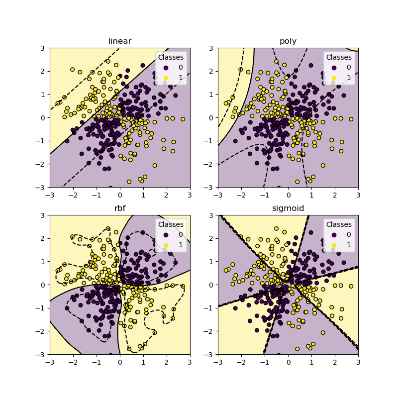
如您從上面的圖表中看到的,只有 rbf 核心可以為上述資料集找到合理的決策邊界。
腳本的總執行時間:(0 分鐘 1.378 秒)
相關範例