使用鄰域成分分析進行降維#

鄰域成分分析在降維中的範例用法。

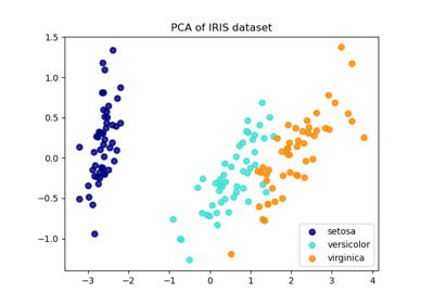
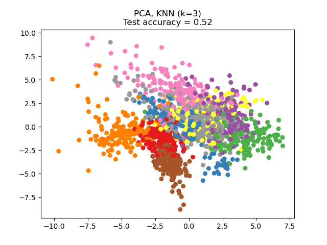
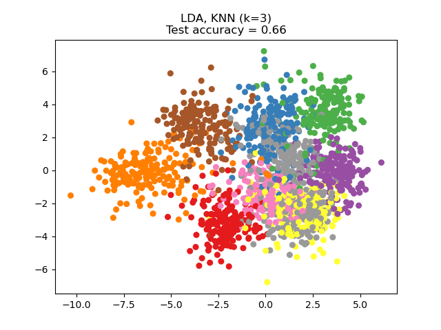
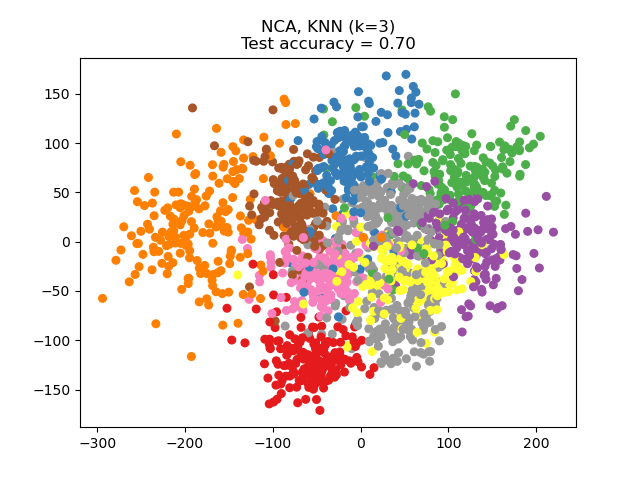
此範例比較應用於數字資料集的不同（線性）降維方法。此資料集包含從 0 到 9 的數字影像，每個類別約有 180 個樣本。每個影像的維度為 8x8 = 64，並縮減為二維資料點。

應用於此資料的主成分分析 (PCA) 識別屬性（主成分，或特徵空間中的方向）的組合，這些組合可以解釋資料中的大部分變異數。在這裡，我們在最前面 2 個主成分上繪製不同的樣本。

線性判別分析 (LDA) 嘗試識別可以解釋類別之間最大變異數的屬性。特別是，與 PCA 相反，LDA 是一種監督方法，使用已知的類別標籤。

鄰域成分分析 (NCA) 嘗試尋找一個特徵空間，使得隨機最近鄰演算法能夠提供最佳的準確性。與 LDA 一樣，它是一種監督方法。

可以看出，儘管維度大幅縮減，NCA 仍強制執行在視覺上有意義的資料聚類。

# Authors: The scikit-learn developers
# SPDX-License-Identifier: BSD-3-Clause

import matplotlib.pyplot as plt
import numpy as np

from sklearn import datasets
from sklearn.decomposition import PCA
from sklearn.discriminant_analysis import LinearDiscriminantAnalysis
from sklearn.model_selection import train_test_split
from sklearn.neighbors import KNeighborsClassifier, NeighborhoodComponentsAnalysis
from sklearn.pipeline import make_pipeline
from sklearn.preprocessing import StandardScaler

n_neighbors = 3
random_state = 0

# Load Digits dataset
X, y = datasets.load_digits(return_X_y=True)

# Split into train/test
X_train, X_test, y_train, y_test = train_test_split(
    X, y, test_size=0.5, stratify=y, random_state=random_state
)

dim = len(X[0])
n_classes = len(np.unique(y))

# Reduce dimension to 2 with PCA
pca = make_pipeline(StandardScaler(), PCA(n_components=2, random_state=random_state))

# Reduce dimension to 2 with LinearDiscriminantAnalysis
lda = make_pipeline(StandardScaler(), LinearDiscriminantAnalysis(n_components=2))

# Reduce dimension to 2 with NeighborhoodComponentAnalysis
nca = make_pipeline(
    StandardScaler(),
    NeighborhoodComponentsAnalysis(n_components=2, random_state=random_state),
)

# Use a nearest neighbor classifier to evaluate the methods
knn = KNeighborsClassifier(n_neighbors=n_neighbors)

# Make a list of the methods to be compared
dim_reduction_methods = [("PCA", pca), ("LDA", lda), ("NCA", nca)]

# plt.figure()
for i, (name, model) in enumerate(dim_reduction_methods):
    plt.figure()
    # plt.subplot(1, 3, i + 1, aspect=1)

    # Fit the method's model
    model.fit(X_train, y_train)

    # Fit a nearest neighbor classifier on the embedded training set
    knn.fit(model.transform(X_train), y_train)

    # Compute the nearest neighbor accuracy on the embedded test set
    acc_knn = knn.score(model.transform(X_test), y_test)

    # Embed the data set in 2 dimensions using the fitted model
    X_embedded = model.transform(X)

    # Plot the projected points and show the evaluation score
    plt.scatter(X_embedded[:, 0], X_embedded[:, 1], c=y, s=30, cmap="Set1")
    plt.title(
        "{}, KNN (k={})\nTest accuracy = {:.2f}".format(name, n_neighbors, acc_knn)
    )
plt.show()