注意
前往結尾 下載完整的範例程式碼。或透過 JupyterLite 或 Binder 在您的瀏覽器中執行此範例
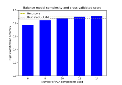
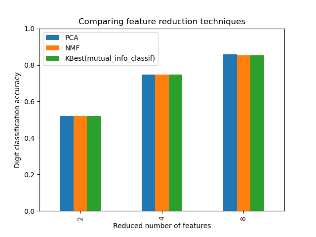
使用 Pipeline 和 GridSearchCV 選擇降維#
此範例建構一個管道,執行降維,然後使用支援向量分類器進行預測。它示範了 GridSearchCV 和 Pipeline 的使用,以在單個 CV 執行中針對不同的估計器類別進行最佳化 – 無監督的 PCA 和 NMF 降維與網格搜尋期間的單變量特徵選擇進行比較。
此外,可以使用 memory 引數來實例化 Pipeline,以記憶管道內的轉換器,避免重複擬合相同的轉換器。
請注意,當轉換器的擬合成本很高時,使用 memory 來啟用快取會變得很有意義。
# Authors: The scikit-learn developers
# SPDX-License-Identifier: BSD-3-Clause
Pipeline 和 GridSearchCV 的圖示#
import matplotlib.pyplot as plt
import numpy as np

from sklearn.datasets import load_digits
from sklearn.decomposition import NMF, PCA
from sklearn.feature_selection import SelectKBest, mutual_info_classif
from sklearn.model_selection import GridSearchCV
from sklearn.pipeline import Pipeline
from sklearn.preprocessing import MinMaxScaler
from sklearn.svm import LinearSVC

X, y = load_digits(return_X_y=True)

pipe = Pipeline(
    [
        ("scaling", MinMaxScaler()),
        # the reduce_dim stage is populated by the param_grid
        ("reduce_dim", "passthrough"),
        ("classify", LinearSVC(dual=False, max_iter=10000)),
    ]
)

N_FEATURES_OPTIONS = [2, 4, 8]
C_OPTIONS = [1, 10, 100, 1000]
param_grid = [
    {
        "reduce_dim": [PCA(iterated_power=7), NMF(max_iter=1_000)],
        "reduce_dim__n_components": N_FEATURES_OPTIONS,
        "classify__C": C_OPTIONS,
    },
    {
        "reduce_dim": [SelectKBest(mutual_info_classif)],
        "reduce_dim__k": N_FEATURES_OPTIONS,
        "classify__C": C_OPTIONS,
    },
]
reducer_labels = ["PCA", "NMF", "KBest(mutual_info_classif)"]

grid = GridSearchCV(pipe, n_jobs=1, param_grid=param_grid)
grid.fit(X, y)
import pandas as pd

mean_scores = np.array(grid.cv_results_["mean_test_score"])
# scores are in the order of param_grid iteration, which is alphabetical
mean_scores = mean_scores.reshape(len(C_OPTIONS), -1, len(N_FEATURES_OPTIONS))
# select score for best C
mean_scores = mean_scores.max(axis=0)
# create a dataframe to ease plotting
mean_scores = pd.DataFrame(
    mean_scores.T, index=N_FEATURES_OPTIONS, columns=reducer_labels
)

ax = mean_scores.plot.bar()
ax.set_title("Comparing feature reduction techniques")
ax.set_xlabel("Reduced number of features")
ax.set_ylabel("Digit classification accuracy")
ax.set_ylim((0, 1))
ax.legend(loc="upper left")

plt.show()
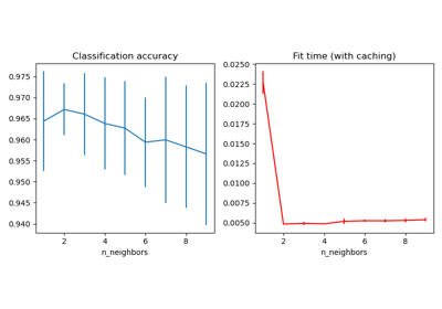
快取 Pipeline 中的轉換器#
有時值得儲存特定轉換器的狀態,因為它可以再次使用。在 GridSearchCV 中使用管道會觸發這種情況。因此,我們使用引數 memory 來啟用快取。
警告
請注意,此範例僅為說明,因為在此特定情況下,擬合 PCA 不一定比載入快取慢。因此,當轉換器的擬合成本很高時,請使用 memory 建構函式參數。
from shutil import rmtree

from joblib import Memory

# Create a temporary folder to store the transformers of the pipeline
location = "cachedir"
memory = Memory(location=location, verbose=10)
cached_pipe = Pipeline(
    [("reduce_dim", PCA()), ("classify", LinearSVC(dual=False, max_iter=10000))],
    memory=memory,
)

# This time, a cached pipeline will be used within the grid search


# Delete the temporary cache before exiting
memory.clear(warn=False)
rmtree(location)
PCA 擬合僅在評估 LinearSVC 分類器的 C 參數的第一個組態時計算。其他 C 組態將觸發載入快取的 PCA 估計器資料,從而節省處理時間。因此,當擬合轉換器的成本很高時,使用 memory 快取管道非常有益。
腳本的總執行時間:(0 分鐘 50.692 秒)
相關範例