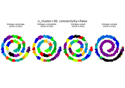
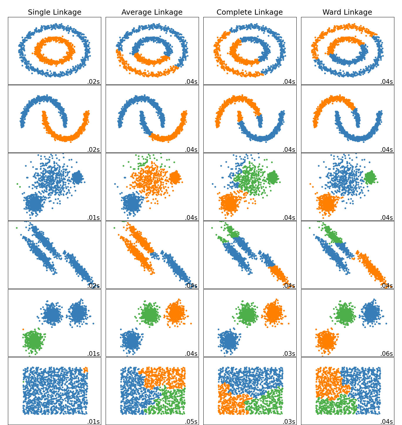
比較玩具資料集上不同的階層式鏈結方法#

此範例展示了在「有趣」但仍然是 2D 的資料集上，階層式叢集的不同鏈結方法的特性。

主要的觀察是

單一鏈結速度快，且在非球狀資料上表現良好，但在存在雜訊的情況下表現不佳。
平均和完整鏈結在乾淨分離的球狀叢集上表現良好，但在其他情況下結果參差不齊。
Ward 是雜訊資料最有效的方法。

雖然這些範例對演算法提供了一些直觀概念，但這種直觀概念可能不適用於非常高維度的資料。

# Authors: The scikit-learn developers
# SPDX-License-Identifier: BSD-3-Clause

import time
import warnings
from itertools import cycle, islice

import matplotlib.pyplot as plt
import numpy as np

from sklearn import cluster, datasets
from sklearn.preprocessing import StandardScaler

產生資料集。我們選擇足夠大的大小來查看演算法的可擴展性，但又不會太大而避免執行時間過長

n_samples = 1500
noisy_circles = datasets.make_circles(
    n_samples=n_samples, factor=0.5, noise=0.05, random_state=170
)
noisy_moons = datasets.make_moons(n_samples=n_samples, noise=0.05, random_state=170)
blobs = datasets.make_blobs(n_samples=n_samples, random_state=170)
rng = np.random.RandomState(170)
no_structure = rng.rand(n_samples, 2), None

# Anisotropicly distributed data
X, y = datasets.make_blobs(n_samples=n_samples, random_state=170)
transformation = [[0.6, -0.6], [-0.4, 0.8]]
X_aniso = np.dot(X, transformation)
aniso = (X_aniso, y)

# blobs with varied variances
varied = datasets.make_blobs(
    n_samples=n_samples, cluster_std=[1.0, 2.5, 0.5], random_state=170
)

執行叢集並繪圖

# Set up cluster parameters
plt.figure(figsize=(9 * 1.3 + 2, 14.5))
plt.subplots_adjust(
    left=0.02, right=0.98, bottom=0.001, top=0.96, wspace=0.05, hspace=0.01
)

plot_num = 1

default_base = {"n_neighbors": 10, "n_clusters": 3}

datasets = [
    (noisy_circles, {"n_clusters": 2}),
    (noisy_moons, {"n_clusters": 2}),
    (varied, {"n_neighbors": 2}),
    (aniso, {"n_neighbors": 2}),
    (blobs, {}),
    (no_structure, {}),
]

for i_dataset, (dataset, algo_params) in enumerate(datasets):
    # update parameters with dataset-specific values
    params = default_base.copy()
    params.update(algo_params)

    X, y = dataset

    # normalize dataset for easier parameter selection
    X = StandardScaler().fit_transform(X)

    # ============
    # Create cluster objects
    # ============
    ward = cluster.AgglomerativeClustering(
        n_clusters=params["n_clusters"], linkage="ward"
    )
    complete = cluster.AgglomerativeClustering(
        n_clusters=params["n_clusters"], linkage="complete"
    )
    average = cluster.AgglomerativeClustering(
        n_clusters=params["n_clusters"], linkage="average"
    )
    single = cluster.AgglomerativeClustering(
        n_clusters=params["n_clusters"], linkage="single"
    )

    clustering_algorithms = (
        ("Single Linkage", single),
        ("Average Linkage", average),
        ("Complete Linkage", complete),
        ("Ward Linkage", ward),
    )

    for name, algorithm in clustering_algorithms:
        t0 = time.time()

        # catch warnings related to kneighbors_graph
        with warnings.catch_warnings():
            warnings.filterwarnings(
                "ignore",
                message="the number of connected components of the "
                + "connectivity matrix is [0-9]{1,2}"
                + " > 1. Completing it to avoid stopping the tree early.",
                category=UserWarning,
            )
            algorithm.fit(X)

        t1 = time.time()
        if hasattr(algorithm, "labels_"):
            y_pred = algorithm.labels_.astype(int)
        else:
            y_pred = algorithm.predict(X)

        plt.subplot(len(datasets), len(clustering_algorithms), plot_num)
        if i_dataset == 0:
            plt.title(name, size=18)

        colors = np.array(
            list(
                islice(
                    cycle(
                        [
                            "#377eb8",
                            "#ff7f00",
                            "#4daf4a",
                            "#f781bf",
                            "#a65628",
                            "#984ea3",
                            "#999999",
                            "#e41a1c",
                            "#dede00",
                        ]
                    ),
                    int(max(y_pred) + 1),
                )
            )
        )
        plt.scatter(X[:, 0], X[:, 1], s=10, color=colors[y_pred])

        plt.xlim(-2.5, 2.5)
        plt.ylim(-2.5, 2.5)
        plt.xticks(())
        plt.yticks(())
        plt.text(
            0.99,
            0.01,
            ("%.2fs" % (t1 - t0)).lstrip("0"),
            transform=plt.gca().transAxes,
            size=15,
            horizontalalignment="right",
        )
        plot_num += 1

plt.show()