比較分類器的校準#

良好校準的分類器是機率分類器，其 predict_proba 的輸出可以直接解釋為信心水準。例如，一個良好校準的（二元）分類器應該對樣本進行分類，使得對於給出 predict_proba 值接近 0.8 的樣本，大約 80% 實際上屬於正類別。

在此範例中，我們將比較四種不同模型的校準：邏輯迴歸、高斯樸素貝葉斯、隨機森林分類器和線性 SVM。

作者：scikit-learn 開發人員 SPDX-License-Identifier：BSD-3-Clause

#
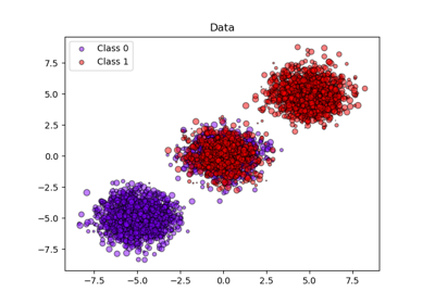
# Dataset
# -------
#
# We will use a synthetic binary classification dataset with 100,000 samples
# and 20 features. Of the 20 features, only 2 are informative, 2 are
# redundant (random combinations of the informative features) and the
# remaining 16 are uninformative (random numbers).
#
# Of the 100,000 samples, 100 will be used for model fitting and the remaining
# for testing. Note that this split is quite unusual: the goal is to obtain
# stable calibration curve estimates for models that are potentially prone to
# overfitting. In practice, one should rather use cross-validation with more
# balanced splits but this would make the code of this example more complicated
# to follow.

from sklearn.datasets import make_classification
from sklearn.model_selection import train_test_split

X, y = make_classification(
    n_samples=100_000, n_features=20, n_informative=2, n_redundant=2, random_state=42
)

train_samples = 100  # Samples used for training the models
X_train, X_test, y_train, y_test = train_test_split(
    X,
    y,
    shuffle=False,
    test_size=100_000 - train_samples,
)

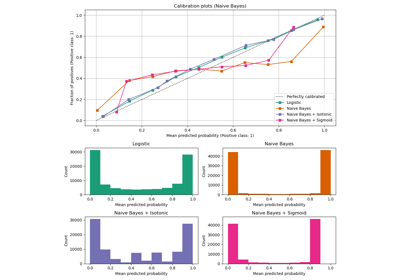
校準曲線#

以下，我們使用小型訓練資料集訓練四種模型中的每一種，然後使用測試資料集的預測機率繪製校準曲線（也稱為可靠性圖）。校準曲線的建立方法是將預測機率分組，然後繪製每個組中的平均預測機率與觀察到的頻率（「正數的比例」）。在校準曲線下方，我們繪製一個直方圖，顯示預測機率的分佈，或者更具體地說，每個預測機率組中的樣本數。

import numpy as np

from sklearn.svm import LinearSVC


class NaivelyCalibratedLinearSVC(LinearSVC):
    """LinearSVC with `predict_proba` method that naively scales
    `decision_function` output."""

    def fit(self, X, y):
        super().fit(X, y)
        df = self.decision_function(X)
        self.df_min_ = df.min()
        self.df_max_ = df.max()

    def predict_proba(self, X):
        """Min-max scale output of `decision_function` to [0,1]."""
        df = self.decision_function(X)
        calibrated_df = (df - self.df_min_) / (self.df_max_ - self.df_min_)
        proba_pos_class = np.clip(calibrated_df, 0, 1)
        proba_neg_class = 1 - proba_pos_class
        proba = np.c_[proba_neg_class, proba_pos_class]
        return proba

from sklearn.calibration import CalibrationDisplay
from sklearn.ensemble import RandomForestClassifier
from sklearn.linear_model import LogisticRegressionCV
from sklearn.naive_bayes import GaussianNB

# Define the classifiers to be compared in the study.
#
# Note that we use a variant of the logistic regression model that can
# automatically tune its regularization parameter.
#
# For a fair comparison, we should run a hyper-parameter search for all the
# classifiers but we don't do it here for the sake of keeping the example code
# concise and fast to execute.
lr = LogisticRegressionCV(
    Cs=np.logspace(-6, 6, 101), cv=10, scoring="neg_log_loss", max_iter=1_000
)
gnb = GaussianNB()
svc = NaivelyCalibratedLinearSVC(C=1.0)
rfc = RandomForestClassifier(random_state=42)

clf_list = [
    (lr, "Logistic Regression"),
    (gnb, "Naive Bayes"),
    (svc, "SVC"),
    (rfc, "Random forest"),
]

import matplotlib.pyplot as plt
from matplotlib.gridspec import GridSpec

fig = plt.figure(figsize=(10, 10))
gs = GridSpec(4, 2)
colors = plt.get_cmap("Dark2")

ax_calibration_curve = fig.add_subplot(gs[:2, :2])
calibration_displays = {}
markers = ["^", "v", "s", "o"]
for i, (clf, name) in enumerate(clf_list):
    clf.fit(X_train, y_train)
    display = CalibrationDisplay.from_estimator(
        clf,
        X_test,
        y_test,
        n_bins=10,
        name=name,
        ax=ax_calibration_curve,
        color=colors(i),
        marker=markers[i],
    )
    calibration_displays[name] = display

ax_calibration_curve.grid()
ax_calibration_curve.set_title("Calibration plots")

# Add histogram
grid_positions = [(2, 0), (2, 1), (3, 0), (3, 1)]
for i, (_, name) in enumerate(clf_list):
    row, col = grid_positions[i]
    ax = fig.add_subplot(gs[row, col])

    ax.hist(
        calibration_displays[name].y_prob,
        range=(0, 1),
        bins=10,
        label=name,
        color=colors(i),
    )
    ax.set(title=name, xlabel="Mean predicted probability", ylabel="Count")

plt.tight_layout()
plt.show()

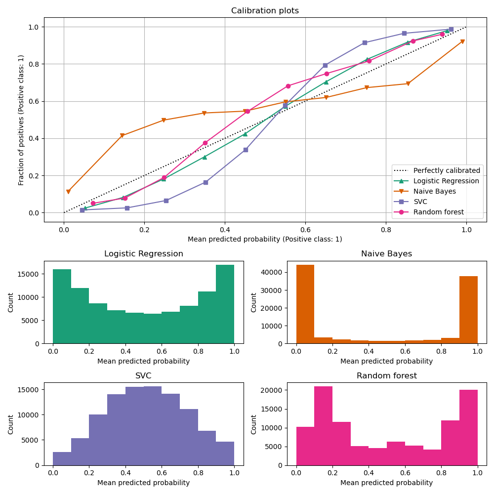
Calibration plots, Logistic Regression, Naive Bayes, SVC, Random forest

結果分析#

LogisticRegressionCV 儘管訓練集大小較小，仍會傳回校準良好的預測：其可靠性曲線在四個模型中是最接近對角線的。

邏輯迴歸的訓練方式是最小化對數損失，這是一種嚴格的適當評分規則：在無限訓練資料的限制下，嚴格的適當評分規則會被預測真實條件機率的模型最小化。因此，（假設的）模型將會被完美校準。然而，使用適當的評分規則作為訓練目標並不足以保證模型本身校準良好：即使有非常大的訓練集，如果邏輯迴歸的正規化過於強烈，或輸入特徵的選擇和預處理導致此模型規格錯誤（例如，如果資料集的真實決策邊界是輸入特徵的高度非線性函數），則邏輯迴歸仍然可能校準不良。

在此範例中，訓練集有意保持非常小。在此設定中，由於過擬合，最佳化對數損失仍可能導致校準不良的模型。為了減輕這種情況，LogisticRegressionCV 類別已設定為調整 C 正規化參數，以便透過內部交叉驗證最小化對數損失，從而在此小型訓練集設定中找到此模型的最佳折衷方案。

由於訓練集的大小有限且缺乏良好規格的保證，我們觀察到邏輯迴歸模型的校準曲線接近但並非完美位於對角線上。此模型的校準曲線形狀可以解釋為稍微過於不自信：相較於正樣本的真實比例，預測機率有點太接近 0.5。

其他方法都輸出校準較差的機率

GaussianNB 傾向於將此特定資料集上的機率推向 0 或 1（請參閱直方圖）（過度自信）。這主要是因為樸素貝葉斯方程式只有在特徵條件獨立的假設成立時才能提供正確的機率估計[2]。然而，特徵可能是相關的，而這種情況就是這個資料集的情況，其中包含 2 個特徵，這些特徵是作為資訊豐富的特徵的隨機線性組合而產生的。這些相關的特徵實際上被「計算了兩次」，導致預測機率趨向於 0 和 1 [3]。但是請注意，更改用於產生資料集的種子可能會導致樸素貝葉斯估計器的結果差異很大。
LinearSVC 本身並非自然的機率分類器。為了將其預測解釋為機率分類器，我們天真地將 decision_function 的輸出透過在上面定義的 NaivelyCalibratedLinearSVC 包裝器類別中應用最小-最大縮放縮放為 [0, 1]。此估計器在此資料上顯示典型的 S 形校準曲線：大於 0.5 的預測對應於有效正類別比例甚至更大的樣本（在對角線上方），而小於 0.5 的預測對應於正類別比例更小的樣本（在對角線下方）。這種不自信的預測對於最大邊界方法而言很典型[1]。
RandomForestClassifier 的預測直方圖顯示在約 0.2 和 0.9 機率處有峰值，而接近 0 或 1 的機率非常罕見。 [1] 給出了對此的解釋：「諸如 bagging 和隨機森林等方法會對基礎模型集合的預測結果進行平均，因此難以做出接近 0 和 1 的預測，因為基礎模型中的變異性會使預測結果偏離接近零或一的值。由於預測結果被限制在 [0, 1] 的區間內，因此由變異性引起的誤差往往在接近零和一時是單邊的。例如，如果模型應該預測某個案例的 p = 0，那麼 bagging 實現這一點的唯一方法是所有 bagging 的樹都預測為零。如果我們在 bagging 平均的樹中加入雜訊，這種雜訊會導致某些樹預測該案例的值大於 0，從而使 bagging 整合的平均預測值偏離 0。我們在隨機森林中觀察到這種效應最為強烈，因為使用隨機森林訓練的基層樹由於特徵子集化而具有相對較高的變異性。」這種效應會使隨機森林變得過於不自信。儘管存在這種可能的偏差，但請注意，這些樹本身是透過最小化 Gini 或 Entropy 標準來擬合的，這兩者都會導致最小化適當評分規則的拆分：分別是 Brier 分數或對數損失。有關更多詳細資訊，請參閱使用者指南。這可以解釋為什麼此模型在此特定範例資料集上顯示出足夠好的校準曲線。事實上，隨機森林模型的不自信程度並未明顯高於 Logistic 回歸模型。

隨時可以重新執行此範例，使用不同的隨機種子和其他資料集生成參數，以查看校準圖的外觀有何不同。一般來說，Logistic 回歸和隨機森林往往是校準最佳的分類器，而 SVC 則經常顯示出典型的不自信校準不足。樸素貝葉斯模型通常校準也很差，但其校準曲線的總體形狀會因資料集而異。

最後，請注意，對於某些資料集種子，即使像上面一樣調整正規化參數，所有模型的校準效果都很差。當訓練規模太小或模型嚴重錯誤指定時，這種情況勢必會發生。

參考文獻#

腳本的總執行時間：(0 分鐘 2.900 秒)

相關範例

機率校準曲線

分類器的機率校準

三類分類的機率校準

繪製 VotingClassifier 計算的類別機率

由 Sphinx-Gallery 產生的圖庫