注意
前往結尾下載完整的範例程式碼。或透過 JupyterLite 或 Binder 在您的瀏覽器中執行此範例
事後調整成本敏感學習的決策閾值#
一旦訓練好分類器,predict 方法的輸出會輸出與 decision_function 或 predict_proba 輸出閾值處理相對應的類別標籤預測。對於二元分類器,預設閾值定義為後驗機率估計值 0.5 或決策分數 0.0。
然而,這種預設策略很可能不是手邊任務的最佳選擇。在這裡,我們使用「Statlog」德國信貸資料集 [1] 來展示一個使用案例。在此資料集中,任務是預測一個人是否具有「良好」或「不良」的信譽。此外,還提供了一個成本矩陣,指定錯誤分類的成本。具體來說,將「不良」信譽錯誤分類為「良好」的平均成本是將「良好」信譽錯誤分類為「不良」的五倍。
我們使用 TunedThresholdClassifierCV 來選擇決策函數的截止點,以最小化所提供的業務成本。
在範例的第二部分中,我們透過考慮信用卡交易中的詐欺檢測問題來進一步擴展這種方法:在這種情況下,業務指標取決於每筆個別交易的金額。
參考文獻
# Authors: The scikit-learn developers
# SPDX-License-Identifier: BSD-3-Clause
具有固定收益和成本的成本敏感學習#
在第一部分中,我們說明在混淆矩陣的每個條目相關的收益和成本為常數的情況下使用 TunedThresholdClassifierCV 的方式。我們使用 [2] 中提出的問題,並使用「Statlog」德國信貸資料集 [1]。
「Statlog」德國信貸資料集#
我們從 OpenML 取得德國信貸資料集。
import sklearn
from sklearn.datasets import fetch_openml

sklearn.set_config(transform_output="pandas")

german_credit = fetch_openml(data_id=31, as_frame=True, parser="pandas")
X, y = german_credit.data, german_credit.target
我們檢查 X 中可用的特徵類型。
X.info()
<class 'pandas.core.frame.DataFrame'>
RangeIndex: 1000 entries, 0 to 999
Data columns (total 20 columns):
 #   Column                  Non-Null Count  Dtype
---  ------                  --------------  -----
 0   checking_status         1000 non-null   category
 1   duration                1000 non-null   int64
 2   credit_history          1000 non-null   category
 3   purpose                 1000 non-null   category
 4   credit_amount           1000 non-null   int64
 5   savings_status          1000 non-null   category
 6   employment              1000 non-null   category
 7   installment_commitment  1000 non-null   int64
 8   personal_status         1000 non-null   category
 9   other_parties           1000 non-null   category
 10  residence_since         1000 non-null   int64
 11  property_magnitude      1000 non-null   category
 12  age                     1000 non-null   int64
 13  other_payment_plans     1000 non-null   category
 14  housing                 1000 non-null   category
 15  existing_credits        1000 non-null   int64
 16  job                     1000 non-null   category
 17  num_dependents          1000 non-null   int64
 18  own_telephone           1000 non-null   category
 19  foreign_worker          1000 non-null   category
dtypes: category(13), int64(7)
memory usage: 69.9 KB
許多特徵是類別的,而且通常使用字串編碼。當我們開發預測模型時,需要對這些類別進行編碼。讓我們檢查目標。
y.value_counts()
class
good    700
bad     300
Name: count, dtype: int64
另一個觀察結果是,資料集是不平衡的。在評估我們的預測模型時,我們需要謹慎,並使用一組適用於這種情況的指標。
此外,我們觀察到目標是使用字串編碼的。某些指標(例如精確率和召回率)也需要提供感興趣的標籤,也稱為「正向標籤」。在這裡,我們定義我們的目標是預測樣本是否為「不良」信譽。
pos_label, neg_label = "bad", "good"
為了執行我們的分析,我們使用單一分層分割來分割我們的資料集。
from sklearn.model_selection import train_test_split

X_train, X_test, y_train, y_test = train_test_split(X, y, stratify=y, random_state=0)
我們已準備好設計我們的預測模型和相關的評估策略。
評估指標#
在本節中,我們定義一組稍後會使用的指標。為了查看調整截止點的效果,我們使用接受者操作特徵 (ROC) 曲線和精確率-召回率曲線來評估預測模型。因此,這些圖表上報告的值是真陽性率 (TPR),也稱為召回率或靈敏度,以及假陽性率 (FPR),也稱為 ROC 曲線的特異性,以及精確率-召回率曲線的精確率和召回率。
從這四個指標來看,scikit-learn 沒有提供 FPR 的評分器。因此,我們需要定義一個小型的自訂函數來計算它。
from sklearn.metrics import confusion_matrix


def fpr_score(y, y_pred, neg_label, pos_label):
    cm = confusion_matrix(y, y_pred, labels=[neg_label, pos_label])
    tn, fp, _, _ = cm.ravel()
    tnr = tn / (tn + fp)
    return 1 - tnr
如先前所述,「正向標籤」未定義為值「1」,並且使用此非標準值呼叫某些指標會引發錯誤。我們需要將「正向標籤」的指示提供給指標。
因此,我們需要使用 make_scorer 定義 scikit-learn 評分器,其中會傳遞資訊。我們將所有自訂評分器儲存在字典中。若要使用它們,我們需要傳遞擬合的模型、資料和我們要評估預測模型所依據的目標。
from sklearn.metrics import make_scorer, precision_score, recall_score

tpr_score = recall_score  # TPR and recall are the same metric
scoring = {
    "precision": make_scorer(precision_score, pos_label=pos_label),
    "recall": make_scorer(recall_score, pos_label=pos_label),
    "fpr": make_scorer(fpr_score, neg_label=neg_label, pos_label=pos_label),
    "tpr": make_scorer(tpr_score, pos_label=pos_label),
}
此外,原始研究 [1] 定義了一個自訂業務指標。我們將「業務指標」稱為任何旨在量化預測(正確或錯誤)如何影響在特定應用程式情境中部署指定機器學習模型的業務價值的指標函數。對於我們的信用預測任務,作者提供了一個自訂成本矩陣,其中編碼將「不良」信譽分類為「良好」的成本平均高出 5 倍,而不是相反:對於融資機構來說,不向一個不會違約的潛在客戶提供信貸(因此錯失一個本來會償還信貸並支付利息的優良客戶)的成本低於向一個會違約的客戶提供信貸。
我們定義一個 python 函數,該函數權衡混淆矩陣並返回總體成本。
import numpy as np


def credit_gain_score(y, y_pred, neg_label, pos_label):
    cm = confusion_matrix(y, y_pred, labels=[neg_label, pos_label])
    # The rows of the confusion matrix hold the counts of observed classes
    # while the columns hold counts of predicted classes. Recall that here we
    # consider "bad" as the positive class (second row and column).
    # Scikit-learn model selection tools expect that we follow a convention
    # that "higher" means "better", hence the following gain matrix assigns
    # negative gains (costs) to the two kinds of prediction errors:
    # - a gain of -1 for each false positive ("good" credit labeled as "bad"),
    # - a gain of -5 for each false negative ("bad" credit labeled as "good"),
    # The true positives and true negatives are assigned null gains in this
    # metric.
    #
    # Note that theoretically, given that our model is calibrated and our data
    # set representative and large enough, we do not need to tune the
    # threshold, but can safely set it to the cost ration 1/5, as stated by Eq.
    # (2) in Elkan paper [2]_.
    gain_matrix = np.array(
        [
            [0, -1],  # -1 gain for false positives
            [-5, 0],  # -5 gain for false negatives
        ]
    )
    return np.sum(cm * gain_matrix)


scoring["credit_gain"] = make_scorer(
    credit_gain_score, neg_label=neg_label, pos_label=pos_label
)
原始預測模型#
我們使用 HistGradientBoostingClassifier 作為預測模型,它可以原生處理類別特徵和遺失值。
from sklearn.ensemble import HistGradientBoostingClassifier

model = HistGradientBoostingClassifier(
    categorical_features="from_dtype", random_state=0
).fit(X_train, y_train)
model
我們使用 ROC 和精確率-召回率曲線來評估預測模型的效能。
import matplotlib.pyplot as plt

from sklearn.metrics import PrecisionRecallDisplay, RocCurveDisplay

fig, axs = plt.subplots(nrows=1, ncols=2, figsize=(14, 6))

PrecisionRecallDisplay.from_estimator(
    model, X_test, y_test, pos_label=pos_label, ax=axs[0], name="GBDT"
)
axs[0].plot(
    scoring["recall"](model, X_test, y_test),
    scoring["precision"](model, X_test, y_test),
    marker="o",
    markersize=10,
    color="tab:blue",
    label="Default cut-off point at a probability of 0.5",
)
axs[0].set_title("Precision-Recall curve")
axs[0].legend()

RocCurveDisplay.from_estimator(
    model,
    X_test,
    y_test,
    pos_label=pos_label,
    ax=axs[1],
    name="GBDT",
    plot_chance_level=True,
)
axs[1].plot(
    scoring["fpr"](model, X_test, y_test),
    scoring["tpr"](model, X_test, y_test),
    marker="o",
    markersize=10,
    color="tab:blue",
    label="Default cut-off point at a probability of 0.5",
)
axs[1].set_title("ROC curve")
axs[1].legend()
_ = fig.suptitle("Evaluation of the vanilla GBDT model")
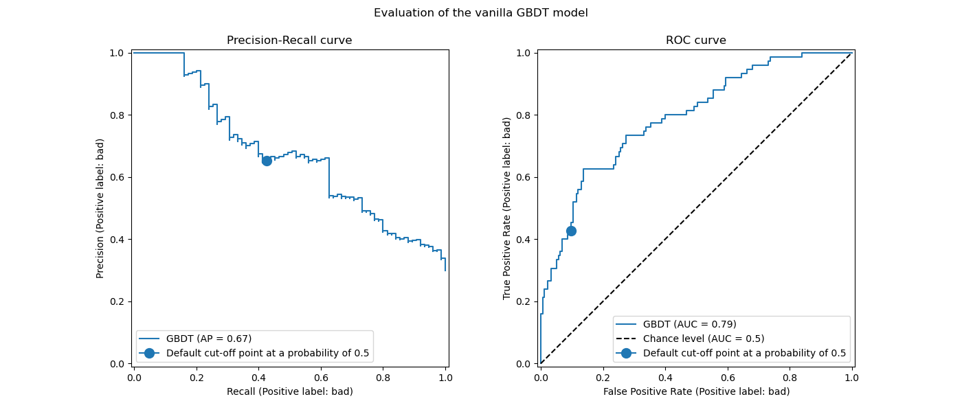
我們回顧一下,這些曲線提供了預測模型在不同截斷點下的統計效能洞察。對於精確率-召回率曲線,報告的指標是精確率和召回率,對於 ROC 曲線,報告的指標是 TPR(與召回率相同)和 FPR。
在此,不同的截斷點對應於介於 0 和 1 之間的不同後驗機率估計值。預設情況下,model.predict 使用機率估計值為 0.5 的截斷點。此類截斷點的指標以曲線上藍色點報告:它對應於使用 model.predict 時模型的統計效能。
然而,我們回顧一下,最初的目的是最小化成本(或最大化收益),如業務指標所定義。我們可以計算業務指標的值
print(f"Business defined metric: {scoring['credit_gain'](model, X_test, y_test)}")
Business defined metric: -232
在此階段,我們不知道是否有任何其他截斷點可以帶來更大的收益。為了找到最佳截斷點,我們需要計算所有可能的截斷點的成本收益,並選擇最佳的截斷點。這個策略手動實作起來可能很繁瑣,但是 TunedThresholdClassifierCV 類別可以幫助我們。它會自動計算所有可能的截斷點的成本收益,並針對 scoring 進行優化。
調整截斷點#
我們使用 TunedThresholdClassifierCV 來調整截斷點。我們需要提供要優化的業務指標以及正標籤。在內部,會選擇最佳截斷點,使其透過交叉驗證最大化業務指標。預設情況下,使用 5 折分層交叉驗證。
from sklearn.model_selection import TunedThresholdClassifierCV

tuned_model = TunedThresholdClassifierCV(
    estimator=model,
    scoring=scoring["credit_gain"],
    store_cv_results=True,  # necessary to inspect all results
)
tuned_model.fit(X_train, y_train)
print(f"{tuned_model.best_threshold_=:0.2f}")
tuned_model.best_threshold_=0.02
我們繪製原始模型和調整模型之 ROC 和精確率-召回率曲線。我們也繪製每個模型將使用的截斷點。因為我們稍後會重複使用相同的程式碼,因此我們定義一個產生繪圖的函式。
def plot_roc_pr_curves(vanilla_model, tuned_model, *, title):
    fig, axs = plt.subplots(nrows=1, ncols=3, figsize=(21, 6))

    linestyles = ("dashed", "dotted")
    markerstyles = ("o", ">")
    colors = ("tab:blue", "tab:orange")
    names = ("Vanilla GBDT", "Tuned GBDT")
    for idx, (est, linestyle, marker, color, name) in enumerate(
        zip((vanilla_model, tuned_model), linestyles, markerstyles, colors, names)
    ):
        decision_threshold = getattr(est, "best_threshold_", 0.5)
        PrecisionRecallDisplay.from_estimator(
            est,
            X_test,
            y_test,
            pos_label=pos_label,
            linestyle=linestyle,
            color=color,
            ax=axs[0],
            name=name,
        )
        axs[0].plot(
            scoring["recall"](est, X_test, y_test),
            scoring["precision"](est, X_test, y_test),
            marker,
            markersize=10,
            color=color,
            label=f"Cut-off point at probability of {decision_threshold:.2f}",
        )
        RocCurveDisplay.from_estimator(
            est,
            X_test,
            y_test,
            pos_label=pos_label,
            linestyle=linestyle,
            color=color,
            ax=axs[1],
            name=name,
            plot_chance_level=idx == 1,
        )
        axs[1].plot(
            scoring["fpr"](est, X_test, y_test),
            scoring["tpr"](est, X_test, y_test),
            marker,
            markersize=10,
            color=color,
            label=f"Cut-off point at probability of {decision_threshold:.2f}",
        )

    axs[0].set_title("Precision-Recall curve")
    axs[0].legend()
    axs[1].set_title("ROC curve")
    axs[1].legend()

    axs[2].plot(
        tuned_model.cv_results_["thresholds"],
        tuned_model.cv_results_["scores"],
        color="tab:orange",
    )
    axs[2].plot(
        tuned_model.best_threshold_,
        tuned_model.best_score_,
        "o",
        markersize=10,
        color="tab:orange",
        label="Optimal cut-off point for the business metric",
    )
    axs[2].legend()
    axs[2].set_xlabel("Decision threshold (probability)")
    axs[2].set_ylabel("Objective score (using cost-matrix)")
    axs[2].set_title("Objective score as a function of the decision threshold")
    fig.suptitle(title)
title = "Comparison of the cut-off point for the vanilla and tuned GBDT model"
plot_roc_pr_curves(model, tuned_model, title=title)
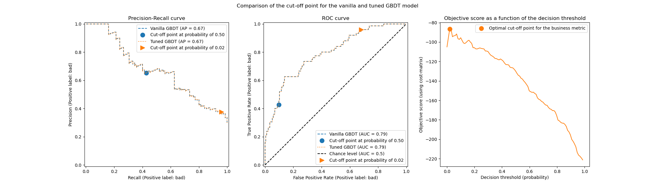
第一個評論是,兩個分類器具有完全相同的 ROC 和精確率-召回率曲線。這是預期的,因為預設情況下,分類器會擬合到相同的訓練資料。在後續章節中,我們將更詳細地討論關於模型重新擬合和交叉驗證的可用選項。
第二個評論是,原始模型和調整模型的截斷點不同。為了了解為何調整模型選擇這個截斷點,我們可以查看右側的圖,其中繪製目標分數,目標分數與我們的業務指標完全相同。我們看到最佳門檻值對應於目標分數的最大值。這個最大值是在遠低於 0.5 的決策門檻值時達到的:調整模型以顯著降低的精確率為代價,享有更高的召回率:調整模型更積極地將「壞」類別標籤預測給更大比例的個人。
我們現在可以檢查選擇此截斷點是否會在測試集上產生更好的分數
print(f"Business defined metric: {scoring['credit_gain'](tuned_model, X_test, y_test)}")
Business defined metric: -134
我們觀察到調整決策門檻值幾乎可以將我們的業務收益提高 2 倍。
關於模型重新擬合和交叉驗證的考量#
在上面的實驗中,我們使用了 TunedThresholdClassifierCV 的預設設定。特別是,截斷點是使用 5 折分層交叉驗證進行調整的。此外,一旦選擇了截斷點,基礎預測模型就會在整個訓練資料上重新擬合。
可以透過提供 refit 和 cv 參數來變更這兩個策略。例如,可以提供擬合的 estimator 並設定 cv="prefit",在這種情況下,截斷點是在擬合時提供的整個資料集上找到的。此外,透過設定 refit=False,基礎分類器不會重新擬合。在這裡,我們可以嘗試做這樣的實驗。
model.fit(X_train, y_train)
tuned_model.set_params(cv="prefit", refit=False).fit(X_train, y_train)
print(f"{tuned_model.best_threshold_=:0.2f}")
tuned_model.best_threshold_=0.28
然後,我們使用與之前相同的方法評估我們的模型
title = "Tuned GBDT model without refitting and using the entire dataset"
plot_roc_pr_curves(model, tuned_model, title=title)
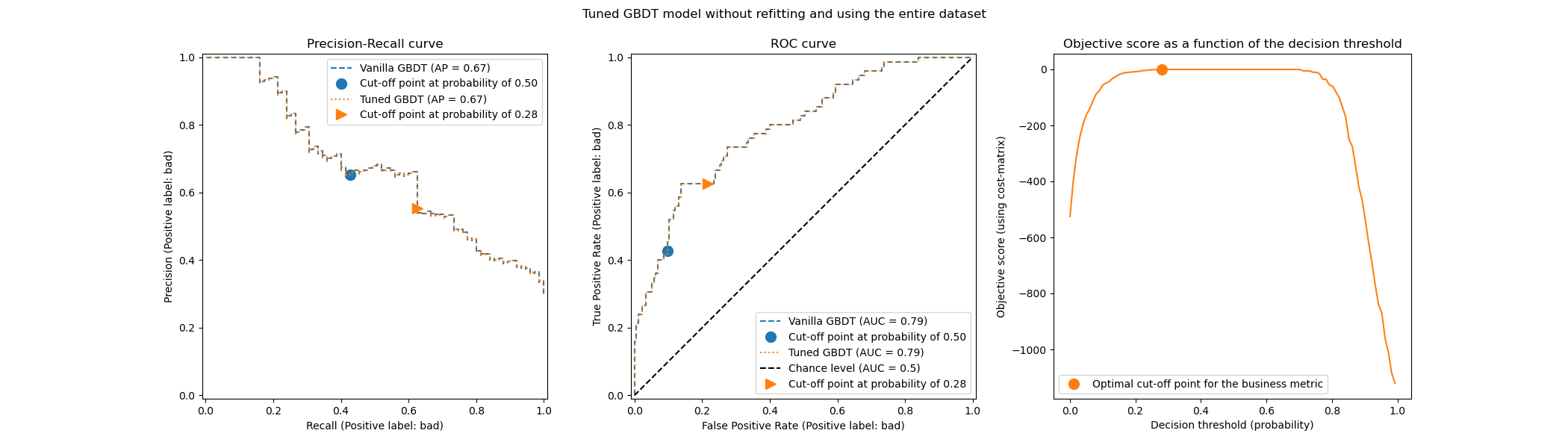
我們觀察到最佳截斷點與先前實驗中找到的截斷點不同。如果我們查看右側的圖,我們會觀察到業務收益在很大範圍的決策門檻值內具有接近最佳 0 收益的較大高原。這種行為是過度擬合的徵兆。由於我們停用了交叉驗證,因此我們在與模型訓練相同的集合上調整了截斷點,這就是觀察到過度擬合的原因。
因此,應謹慎使用此選項。需要確保在擬合時提供給 TunedThresholdClassifierCV 的資料,與用於訓練基礎分類器的資料不同。有時,當想法只是在全新的驗證集上調整預測模型,而無需耗費成本的完整重新擬合時,可能會發生這種情況。
當交叉驗證成本過高時,一種可能的替代方法是,透過將範圍 [0, 1] 中的浮點數提供給 cv 參數,來使用單一的訓練測試拆分。它將資料拆分為訓練集和測試集。讓我們探索此選項
tuned_model.set_params(cv=0.75).fit(X_train, y_train)
title = "Tuned GBDT model without refitting and using the entire dataset"
plot_roc_pr_curves(model, tuned_model, title=title)
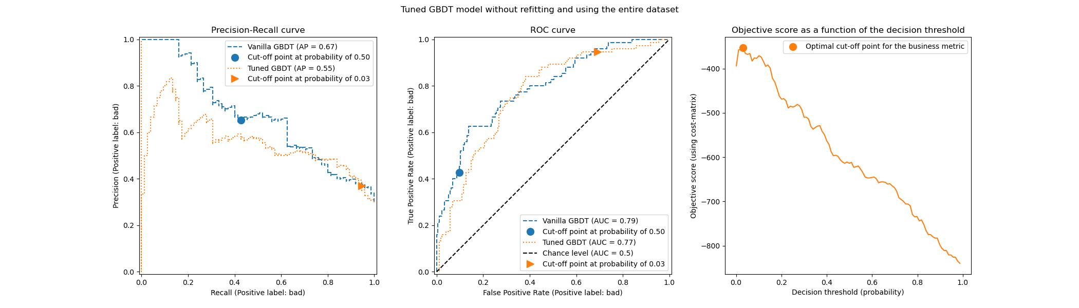
關於截斷點,我們觀察到最佳截斷點與多次重複交叉驗證的情況相似。但是,請注意,單一拆分不考慮擬合/預測過程的變異性,因此我們無法知道截斷點中是否有任何變異。重複交叉驗證會平均消除此影響。
另一個觀察是,調整模型的 ROC 和精確率-召回率曲線。正如預期的那樣,這些曲線與原始模型的曲線不同,因為我們在擬合期間提供的資料子集上訓練了基礎分類器,並保留了驗證集用於調整截斷點。
當收益和成本不是恆定時的成本敏感學習#
如 [2] 中所述,在現實世界的問題中,收益和成本通常不是恆定的。在本節中,我們針對偵測信用卡交易記錄中的詐欺問題,使用與 [2] 中類似的範例。
信用卡資料集#
credit_card = fetch_openml(data_id=1597, as_frame=True, parser="pandas")
credit_card.frame.info()
<class 'pandas.core.frame.DataFrame'>
RangeIndex: 284807 entries, 0 to 284806
Data columns (total 30 columns):
 #   Column  Non-Null Count   Dtype
---  ------  --------------   -----
 0   V1      284807 non-null  float64
 1   V2      284807 non-null  float64
 2   V3      284807 non-null  float64
 3   V4      284807 non-null  float64
 4   V5      284807 non-null  float64
 5   V6      284807 non-null  float64
 6   V7      284807 non-null  float64
 7   V8      284807 non-null  float64
 8   V9      284807 non-null  float64
 9   V10     284807 non-null  float64
 10  V11     284807 non-null  float64
 11  V12     284807 non-null  float64
 12  V13     284807 non-null  float64
 13  V14     284807 non-null  float64
 14  V15     284807 non-null  float64
 15  V16     284807 non-null  float64
 16  V17     284807 non-null  float64
 17  V18     284807 non-null  float64
 18  V19     284807 non-null  float64
 19  V20     284807 non-null  float64
 20  V21     284807 non-null  float64
 21  V22     284807 non-null  float64
 22  V23     284807 non-null  float64
 23  V24     284807 non-null  float64
 24  V25     284807 non-null  float64
 25  V26     284807 non-null  float64
 26  V27     284807 non-null  float64
 27  V28     284807 non-null  float64
 28  Amount  284807 non-null  float64
 29  Class   284807 non-null  category
dtypes: category(1), float64(29)
memory usage: 63.3 MB
資料集包含信用卡記錄的相關資訊,其中一些是詐欺性的,另一些是合法的。因此,目標是預測信用卡記錄是否為詐欺性的。
columns_to_drop = ["Class"]
data = credit_card.frame.drop(columns=columns_to_drop)
target = credit_card.frame["Class"].astype(int)
首先,我們檢查資料集的類別分佈。
target.value_counts(normalize=True)
Class
0    0.998273
1    0.001727
Name: proportion, dtype: float64
資料集高度不平衡,詐欺交易僅佔資料的 0.17%。由於我們有興趣訓練機器學習模型,我們也應該確保在少數類別中有足夠的樣本來訓練模型。
target.value_counts()
Class
0    284315
1       492
Name: count, dtype: int64
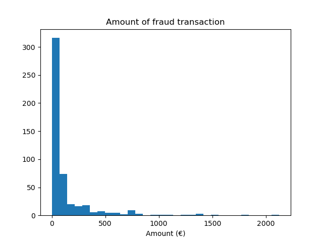
我們觀察到我們有大約 500 個樣本,這在訓練機器學習模型所需的樣本數量方面處於低端。除了目標分佈之外,我們還檢查詐欺交易金額的分佈。
fraud = target == 1
amount_fraud = data["Amount"][fraud]
_, ax = plt.subplots()
ax.hist(amount_fraud, bins=30)
ax.set_title("Amount of fraud transaction")
_ = ax.set_xlabel("Amount (€)")
使用業務指標解決問題#
現在,我們建立一個依賴於每筆交易金額的業務指標。我們定義成本矩陣的方式與 [2] 類似。接受一筆合法的交易可獲得交易金額 2% 的收益。然而,接受一筆詐欺交易將導致交易金額的損失。如 [2] 中所述,拒絕(詐欺和合法交易)的收益和損失並非易於定義。在這裡,我們定義拒絕合法交易的損失估計為 5 歐元,而拒絕詐欺交易的收益估計為 50 歐元。因此,我們定義以下函數來計算給定決策的總收益
def business_metric(y_true, y_pred, amount):
    mask_true_positive = (y_true == 1) & (y_pred == 1)
    mask_true_negative = (y_true == 0) & (y_pred == 0)
    mask_false_positive = (y_true == 0) & (y_pred == 1)
    mask_false_negative = (y_true == 1) & (y_pred == 0)
    fraudulent_refuse = mask_true_positive.sum() * 50
    fraudulent_accept = -amount[mask_false_negative].sum()
    legitimate_refuse = mask_false_positive.sum() * -5
    legitimate_accept = (amount[mask_true_negative] * 0.02).sum()
    return fraudulent_refuse + fraudulent_accept + legitimate_refuse + legitimate_accept
根據此業務指標,我們建立一個 scikit-learn 評分器,該評分器在給定一個已擬合的分類器和一個測試集時,計算業務指標。在這方面,我們使用 make_scorer 工廠。變數 amount 是要傳遞給評分器的額外元數據,我們需要使用 元數據路由 來考慮此資訊。
sklearn.set_config(enable_metadata_routing=True)
business_scorer = make_scorer(business_metric).set_score_request(amount=True)
因此,在此階段,我們觀察到交易金額被使用了兩次:一次作為訓練我們的預測模型的特徵,另一次作為計算業務指標(即模型的統計效能)的元數據。當用作特徵時,我們只需要在 data 中有一個包含每筆交易金額的欄位即可。要將此資訊用作元數據,我們需要有一個外部變數,可以將其傳遞給評分器或模型,以便在內部將此元數據路由到評分器。因此,讓我們建立此變數。
amount = credit_card.frame["Amount"].to_numpy()
from sklearn.model_selection import train_test_split

data_train, data_test, target_train, target_test, amount_train, amount_test = (
    train_test_split(
        data, target, amount, stratify=target, test_size=0.5, random_state=42
    )
)
首先,我們評估一些基準策略以作為參考。回想一下,「0」類別是合法類別,「1」類別是詐欺類別。
from sklearn.dummy import DummyClassifier

always_accept_policy = DummyClassifier(strategy="constant", constant=0)
always_accept_policy.fit(data_train, target_train)
benefit = business_scorer(
    always_accept_policy, data_test, target_test, amount=amount_test
)
print(f"Benefit of the 'always accept' policy: {benefit:,.2f}€")
Benefit of the 'always accept' policy: 221,445.07€
一個將所有交易都視為合法的策略會產生約 220,000 歐元的利潤。我們對一個將所有交易都預測為詐欺的分類器進行相同的評估。
always_reject_policy = DummyClassifier(strategy="constant", constant=1)
always_reject_policy.fit(data_train, target_train)
benefit = business_scorer(
    always_reject_policy, data_test, target_test, amount=amount_test
)
print(f"Benefit of the 'always reject' policy: {benefit:,.2f}€")
Benefit of the 'always reject' policy: -698,490.00€
這樣的策略將會導致災難性的損失:約 670,000 歐元。這是預期的,因為絕大多數交易都是合法的,而該策略將會以不小的成本拒絕它們。
一個根據每筆交易調整接受/拒絕決策的預測模型,理想情況下應該使我們獲得比最佳恆定基準策略的 220,000 歐元更大的利潤。
我們從一個預設決策閾值為 0.5 的邏輯迴歸模型開始。在這裡,我們使用適當的評分規則(對數損失)調整邏輯迴歸的超參數 C,以確保模型通過其 predict_proba 方法返回的機率預測盡可能準確,而不考慮決策閾值的選擇。
from sklearn.linear_model import LogisticRegression
from sklearn.model_selection import GridSearchCV
from sklearn.pipeline import make_pipeline
from sklearn.preprocessing import StandardScaler

logistic_regression = make_pipeline(StandardScaler(), LogisticRegression())
param_grid = {"logisticregression__C": np.logspace(-6, 6, 13)}
model = GridSearchCV(logistic_regression, param_grid, scoring="neg_log_loss").fit(
    data_train, target_train
)
model
print(
    "Benefit of logistic regression with default threshold: "
    f"{business_scorer(model, data_test, target_test, amount=amount_test):,.2f}€"
)
Benefit of logistic regression with default threshold: 244,919.87€
業務指標顯示,我們的預測模型在預設決策閾值下,在利潤方面已經優於基準,並且使用它來接受或拒絕交易將比接受所有交易更有利。
調整決策閾值#
現在的問題是:對於我們想要做出的決策類型,我們的模型是否為最佳?到目前為止,我們還沒有優化決策閾值。我們使用 TunedThresholdClassifierCV 來針對我們的業務評分器優化決策。為了避免巢狀交叉驗證,我們將使用在先前的網格搜尋中找到的最佳估計器。
tuned_model = TunedThresholdClassifierCV(
    estimator=model.best_estimator_,
    scoring=business_scorer,
    thresholds=100,
    n_jobs=2,
)
由於我們的業務評分器需要每筆交易的金額,我們需要在 fit 方法中傳遞此資訊。TunedThresholdClassifierCV 負責自動將此元數據分派給底層評分器。
tuned_model.fit(data_train, target_train, amount=amount_train)
我們觀察到調整後的決策閾值遠離預設值 0.5
print(f"Tuned decision threshold: {tuned_model.best_threshold_:.2f}")
Tuned decision threshold: 0.03
print(
    "Benefit of logistic regression with a tuned threshold: "
    f"{business_scorer(tuned_model, data_test, target_test, amount=amount_test):,.2f}€"
)
Benefit of logistic regression with a tuned threshold: 249,433.39€
我們觀察到,當部署我們的模型時,調整決策閾值會增加預期利潤,如業務指標所示。因此,在可能的情況下,針對業務指標優化決策閾值是有價值的。
手動設定決策閾值,而不是調整它#
在先前的範例中,我們使用 TunedThresholdClassifierCV 來找到最佳決策閾值。然而,在某些情況下,我們可能對手邊的問題有一些先驗知識,並且我們可能很樂意手動設定決策閾值。
類別 FixedThresholdClassifier 允許我們手動設定決策閾值。在預測時,它的行為與先前的調整模型相同,但在擬合過程中不會執行任何搜尋。請注意,在這裡我們使用 FrozenEstimator 來包裝預測模型,以避免任何重新擬合。
在這裡,我們將重新使用上一節中找到的決策閾值來建立一個新模型,並檢查它是否給出相同的結果。
from sklearn.frozen import FrozenEstimator
from sklearn.model_selection import FixedThresholdClassifier

model_fixed_threshold = FixedThresholdClassifier(
    estimator=FrozenEstimator(model), threshold=tuned_model.best_threshold_
)
business_score = business_scorer(
    model_fixed_threshold, data_test, target_test, amount=amount_test
)
print(f"Benefit of logistic regression with a tuned threshold:  {business_score:,.2f}€")
Benefit of logistic regression with a tuned threshold: 249,433.39€
我們觀察到我們得到了完全相同的結果,但是擬合過程要快得多,因為我們沒有執行任何超參數搜尋。
最後,業務指標本身的估計(平均值)可能不可靠,尤其是在少數類別中的資料點數量非常少時。通過對歷史資料進行交叉驗證(離線評估)而估計的任何業務影響,理想情況下應通過對即時資料進行 A/B 測試(線上評估)來確認。但是請注意,A/B 測試模型超出了 scikit-learn 函式庫本身的範圍。
腳本的總執行時間: (0 分鐘 28.508 秒)
相關範例