注意
前往結尾以下載完整的範例程式碼。或透過 JupyterLite 或 Binder 在您的瀏覽器中執行此範例
用於數字分類的限制型波茲曼機特徵#
對於灰階圖像資料,其中像素值可以解釋為白色背景上的黑色程度(例如手寫數字識別),Bernoulli 限制型波茲曼機模型 (BernoulliRBM) 可以執行有效的非線性特徵提取。
# Authors: The scikit-learn developers
# SPDX-License-Identifier: BSD-3-Clause
產生資料#
為了從小型資料集中學習良好的潛在表示法,我們透過在每個方向上以 1 像素的線性位移擾動訓練資料,來人工產生更多標記資料。
import numpy as np
from scipy.ndimage import convolve

from sklearn import datasets
from sklearn.model_selection import train_test_split
from sklearn.preprocessing import minmax_scale


def nudge_dataset(X, Y):
    """
    This produces a dataset 5 times bigger than the original one,
    by moving the 8x8 images in X around by 1px to left, right, down, up
    """
    direction_vectors = [
        [[0, 1, 0], [0, 0, 0], [0, 0, 0]],
        [[0, 0, 0], [1, 0, 0], [0, 0, 0]],
        [[0, 0, 0], [0, 0, 1], [0, 0, 0]],
        [[0, 0, 0], [0, 0, 0], [0, 1, 0]],
    ]

    def shift(x, w):
        return convolve(x.reshape((8, 8)), mode="constant", weights=w).ravel()

    X = np.concatenate(
        [X] + [np.apply_along_axis(shift, 1, X, vector) for vector in direction_vectors]
    )
    Y = np.concatenate([Y for _ in range(5)], axis=0)
    return X, Y


X, y = datasets.load_digits(return_X_y=True)
X = np.asarray(X, "float32")
X, Y = nudge_dataset(X, y)
X = minmax_scale(X, feature_range=(0, 1))  # 0-1 scaling

X_train, X_test, Y_train, Y_test = train_test_split(X, Y, test_size=0.2, random_state=0)
模型定義#
我們建立一個具有 BernoulliRBM 特徵提取器和 LogisticRegression 分類器的分類管道。
from sklearn import linear_model
from sklearn.neural_network import BernoulliRBM
from sklearn.pipeline import Pipeline

logistic = linear_model.LogisticRegression(solver="newton-cg", tol=1)
rbm = BernoulliRBM(random_state=0, verbose=True)

rbm_features_classifier = Pipeline(steps=[("rbm", rbm), ("logistic", logistic)])
訓練#
整個模型(學習率、隱藏層大小、正規化)的超參數透過網格搜尋進行最佳化,但由於執行時間限制,此處不再重複搜尋。
from sklearn.base import clone

# Hyper-parameters. These were set by cross-validation,
# using a GridSearchCV. Here we are not performing cross-validation to
# save time.
rbm.learning_rate = 0.06
rbm.n_iter = 10

# More components tend to give better prediction performance, but larger
# fitting time
rbm.n_components = 100
logistic.C = 6000

# Training RBM-Logistic Pipeline
rbm_features_classifier.fit(X_train, Y_train)

# Training the Logistic regression classifier directly on the pixel
raw_pixel_classifier = clone(logistic)
raw_pixel_classifier.C = 100.0
raw_pixel_classifier.fit(X_train, Y_train)
[BernoulliRBM] Iteration 1, pseudo-likelihood = -25.57, time = 0.11s
[BernoulliRBM] Iteration 2, pseudo-likelihood = -23.68, time = 0.15s
[BernoulliRBM] Iteration 3, pseudo-likelihood = -22.88, time = 0.14s
[BernoulliRBM] Iteration 4, pseudo-likelihood = -21.91, time = 0.14s
[BernoulliRBM] Iteration 5, pseudo-likelihood = -21.79, time = 0.17s
[BernoulliRBM] Iteration 6, pseudo-likelihood = -20.96, time = 0.13s
[BernoulliRBM] Iteration 7, pseudo-likelihood = -20.88, time = 0.13s
[BernoulliRBM] Iteration 8, pseudo-likelihood = -20.50, time = 0.16s
[BernoulliRBM] Iteration 9, pseudo-likelihood = -20.34, time = 0.15s
[BernoulliRBM] Iteration 10, pseudo-likelihood = -20.21, time = 0.14s
評估#
from sklearn import metrics

Y_pred = rbm_features_classifier.predict(X_test)
print(
    "Logistic regression using RBM features:\n%s\n"
    % (metrics.classification_report(Y_test, Y_pred))
)
/home/circleci/project/sklearn/metrics/_classification.py:1565: UndefinedMetricWarning:

Precision is ill-defined and being set to 0.0 in labels with no predicted samples. Use `zero_division` parameter to control this behavior.

/home/circleci/project/sklearn/metrics/_classification.py:1565: UndefinedMetricWarning:

Precision is ill-defined and being set to 0.0 in labels with no predicted samples. Use `zero_division` parameter to control this behavior.

/home/circleci/project/sklearn/metrics/_classification.py:1565: UndefinedMetricWarning:

Precision is ill-defined and being set to 0.0 in labels with no predicted samples. Use `zero_division` parameter to control this behavior.

Logistic regression using RBM features:
              precision    recall  f1-score   support

           0       0.10      1.00      0.18       174
           1       0.00      0.00      0.00       184
           2       0.00      0.00      0.00       166
           3       0.00      0.00      0.00       194
           4       0.00      0.00      0.00       186
           5       0.00      0.00      0.00       181
           6       0.00      0.00      0.00       207
           7       0.00      0.00      0.00       154
           8       0.00      0.00      0.00       182
           9       0.00      0.00      0.00       169

    accuracy                           0.10      1797
   macro avg       0.01      0.10      0.02      1797
weighted avg       0.01      0.10      0.02      1797
Y_pred = raw_pixel_classifier.predict(X_test)
print(
    "Logistic regression using raw pixel features:\n%s\n"
    % (metrics.classification_report(Y_test, Y_pred))
)
/home/circleci/project/sklearn/metrics/_classification.py:1565: UndefinedMetricWarning:

Precision is ill-defined and being set to 0.0 in labels with no predicted samples. Use `zero_division` parameter to control this behavior.

/home/circleci/project/sklearn/metrics/_classification.py:1565: UndefinedMetricWarning:

Precision is ill-defined and being set to 0.0 in labels with no predicted samples. Use `zero_division` parameter to control this behavior.

/home/circleci/project/sklearn/metrics/_classification.py:1565: UndefinedMetricWarning:

Precision is ill-defined and being set to 0.0 in labels with no predicted samples. Use `zero_division` parameter to control this behavior.

Logistic regression using raw pixel features:
              precision    recall  f1-score   support

           0       0.10      1.00      0.18       174
           1       0.00      0.00      0.00       184
           2       0.00      0.00      0.00       166
           3       0.00      0.00      0.00       194
           4       0.00      0.00      0.00       186
           5       0.00      0.00      0.00       181
           6       0.00      0.00      0.00       207
           7       0.00      0.00      0.00       154
           8       0.00      0.00      0.00       182
           9       0.00      0.00      0.00       169

    accuracy                           0.10      1797
   macro avg       0.01      0.10      0.02      1797
weighted avg       0.01      0.10      0.02      1797
相較於原始像素上的邏輯迴歸,BernoulliRBM 提取的特徵有助於提高分類準確度。
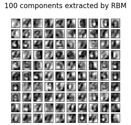
繪圖#
import matplotlib.pyplot as plt

plt.figure(figsize=(4.2, 4))
for i, comp in enumerate(rbm.components_):
    plt.subplot(10, 10, i + 1)
    plt.imshow(comp.reshape((8, 8)), cmap=plt.cm.gray_r, interpolation="nearest")
    plt.xticks(())
    plt.yticks(())
plt.suptitle("100 components extracted by RBM", fontsize=16)
plt.subplots_adjust(0.08, 0.02, 0.92, 0.85, 0.08, 0.23)

plt.show()
腳本的總執行時間: (0 分鐘 3.104 秒)
相關範例