梯度提升袋外估計#

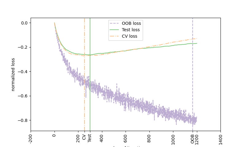
袋外 (OOB) 估計值可以用作估計提升迭代「最佳」數量的有用啟發式方法。OOB 估計值幾乎與交叉驗證估計值相同，但可以即時計算，而無需重複模型擬合。OOB 估計值僅適用於隨機梯度提升（即 subsample < 1.0），估計值是從未包含在自舉樣本中的範例（所謂的袋外範例）的損失改進中得出。OOB 估計器是真實測試損失的悲觀估計器，但對於少量的樹仍然是相當好的近似值。該圖顯示了負 OOB 改進的累計總和，作為提升迭代的函數。如您所見，它在前一百次迭代中追蹤測試損失，但隨後以悲觀的方式發散。該圖還顯示了 3 折交叉驗證的效能，它通常能更好地估計測試損失，但計算量更大。

Accuracy: 0.6860

# Authors: The scikit-learn developers
# SPDX-License-Identifier: BSD-3-Clause

import matplotlib.pyplot as plt
import numpy as np
from scipy.special import expit

from sklearn import ensemble
from sklearn.metrics import log_loss
from sklearn.model_selection import KFold, train_test_split

# Generate data (adapted from G. Ridgeway's gbm example)
n_samples = 1000
random_state = np.random.RandomState(13)
x1 = random_state.uniform(size=n_samples)
x2 = random_state.uniform(size=n_samples)
x3 = random_state.randint(0, 4, size=n_samples)

p = expit(np.sin(3 * x1) - 4 * x2 + x3)
y = random_state.binomial(1, p, size=n_samples)

X = np.c_[x1, x2, x3]

X = X.astype(np.float32)
X_train, X_test, y_train, y_test = train_test_split(X, y, test_size=0.5, random_state=9)

# Fit classifier with out-of-bag estimates
params = {
    "n_estimators": 1200,
    "max_depth": 3,
    "subsample": 0.5,
    "learning_rate": 0.01,
    "min_samples_leaf": 1,
    "random_state": 3,
}
clf = ensemble.GradientBoostingClassifier(**params)

clf.fit(X_train, y_train)
acc = clf.score(X_test, y_test)
print("Accuracy: {:.4f}".format(acc))

n_estimators = params["n_estimators"]
x = np.arange(n_estimators) + 1


def heldout_score(clf, X_test, y_test):
    """compute deviance scores on ``X_test`` and ``y_test``."""
    score = np.zeros((n_estimators,), dtype=np.float64)
    for i, y_proba in enumerate(clf.staged_predict_proba(X_test)):
        score[i] = 2 * log_loss(y_test, y_proba[:, 1])
    return score


def cv_estimate(n_splits=None):
    cv = KFold(n_splits=n_splits)
    cv_clf = ensemble.GradientBoostingClassifier(**params)
    val_scores = np.zeros((n_estimators,), dtype=np.float64)
    for train, test in cv.split(X_train, y_train):
        cv_clf.fit(X_train[train], y_train[train])
        val_scores += heldout_score(cv_clf, X_train[test], y_train[test])
    val_scores /= n_splits
    return val_scores


# Estimate best n_estimator using cross-validation
cv_score = cv_estimate(3)

# Compute best n_estimator for test data
test_score = heldout_score(clf, X_test, y_test)

# negative cumulative sum of oob improvements
cumsum = -np.cumsum(clf.oob_improvement_)

# min loss according to OOB
oob_best_iter = x[np.argmin(cumsum)]

# min loss according to test (normalize such that first loss is 0)
test_score -= test_score[0]
test_best_iter = x[np.argmin(test_score)]

# min loss according to cv (normalize such that first loss is 0)
cv_score -= cv_score[0]
cv_best_iter = x[np.argmin(cv_score)]

# color brew for the three curves
oob_color = list(map(lambda x: x / 256.0, (190, 174, 212)))
test_color = list(map(lambda x: x / 256.0, (127, 201, 127)))
cv_color = list(map(lambda x: x / 256.0, (253, 192, 134)))

# line type for the three curves
oob_line = "dashed"
test_line = "solid"
cv_line = "dashdot"

# plot curves and vertical lines for best iterations
plt.figure(figsize=(8, 4.8))
plt.plot(x, cumsum, label="OOB loss", color=oob_color, linestyle=oob_line)
plt.plot(x, test_score, label="Test loss", color=test_color, linestyle=test_line)
plt.plot(x, cv_score, label="CV loss", color=cv_color, linestyle=cv_line)
plt.axvline(x=oob_best_iter, color=oob_color, linestyle=oob_line)
plt.axvline(x=test_best_iter, color=test_color, linestyle=test_line)
plt.axvline(x=cv_best_iter, color=cv_color, linestyle=cv_line)

# add three vertical lines to xticks
xticks = plt.xticks()
xticks_pos = np.array(
    xticks[0].tolist() + [oob_best_iter, cv_best_iter, test_best_iter]
)
xticks_label = np.array(list(map(lambda t: int(t), xticks[0])) + ["OOB", "CV", "Test"])
ind = np.argsort(xticks_pos)
xticks_pos = xticks_pos[ind]
xticks_label = xticks_label[ind]
plt.xticks(xticks_pos, xticks_label, rotation=90)

plt.legend(loc="upper center")
plt.ylabel("normalized loss")
plt.xlabel("number of iterations")

plt.show()