注意
前往結尾以下載完整的範例程式碼。或透過 JupyterLite 或 Binder 在您的瀏覽器中執行此範例
精確率-召回率#
使用精確率-召回率指標評估分類器輸出品質的範例。
當類別非常不平衡時,精確率-召回率是衡量預測成功與否的有用指標。在資訊檢索中,精確率是實際傳回項目中相關項目的比例,而召回率是在所有應傳回的項目中傳回項目的比例。「相關性」在這裡指的是被正面標記的項目,即真陽性與假陰性。
精確率 (\(P\)) 定義為真陽性 (\(T_p\)) 的數量除以真陽性加假陽性 (\(F_p\)) 的數量。
召回率 (\(R\)) 定義為真陽性 (\(T_p\)) 的數量除以真陽性加假陰性 (\(F_n\)) 的數量。
精確率-召回率曲線顯示不同閾值下精確率和召回率之間的權衡。曲線下的高面積表示高召回率和高精確率。高精確率是透過在傳回的結果中幾乎沒有假陽性來實現的,而高召回率是透過在相關結果中幾乎沒有假陰性來實現的。兩者的高分數表明分類器正在傳回準確的結果(高精確率),以及傳回大多數所有相關結果(高召回率)。
具有高召回率但低精確率的系統會傳回大多數相關項目,但錯誤標記的傳回結果比例很高。具有高精確率但低召回率的系統則恰恰相反,傳回的相關項目很少,但與實際標籤相比,其大多數預測標籤都是正確的。一個具有高精確率和高召回率的理想系統將會傳回大多數相關項目,並且大多數結果都標記正確。
精確率的定義 (\(\frac{T_p}{T_p + F_p}\)) 顯示降低分類器的閾值可能會增加分母,藉此增加傳回的結果數量。如果先前閾值設定過高,則新結果可能都是真陽性,這將會提高精確率。如果先前的閾值適中或過低,則進一步降低閾值將會引入假陽性,進而降低精確率。
召回率定義為 \(\frac{T_p}{T_p+F_n}\),其中 \(T_p+F_n\) 不取決於分類器閾值。變更分類器閾值只能變更分子 \(T_p\)。降低分類器閾值可能會透過增加真陽性結果的數量來提高召回率。降低閾值也可能使召回率保持不變,而精確率則會波動。因此,精確率不一定會隨著召回率而降低。
可以在圖表的階梯區域中觀察到召回率和精確率之間的關係 - 在這些階梯的邊緣,閾值的微小變化會顯著降低精確率,而召回率僅略有增加。
平均精確率 (AP) 將此類圖表總結為每個閾值下實現的精確率的加權平均值,並以先前閾值召回率的增加量作為權重
\(\text{AP} = \sum_n (R_n - R_{n-1}) P_n\)
其中 \(P_n\) 和 \(R_n\) 是第 n 個閾值下的精確率和召回率。一對 \((R_k, P_k)\) 被稱為操作點。
AP 和操作點下的梯形面積(sklearn.metrics.auc)是總結精確率-召回率曲線的常用方法,會產生不同的結果。請在使用者指南中閱讀更多內容。
精確率-召回率曲線通常用於二元分類,以研究分類器的輸出。為了將精確率-召回率曲線和平均精確率擴展到多類別或多標籤分類,必須將輸出二元化。每個標籤可以繪製一條曲線,但也可以透過將標籤指示器矩陣的每個元素視為二元預測 (微平均) 來繪製精確率-召回率曲線。
注意
# Authors: The scikit-learn developers
# SPDX-License-Identifier: BSD-3-Clause
在二元分類設定中#
資料集和模型#
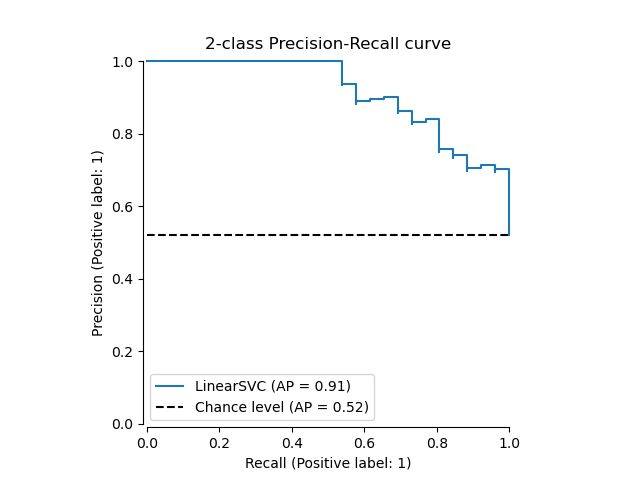
我們將使用線性 SVC 分類器來區分兩種鳶尾花。
import numpy as np

from sklearn.datasets import load_iris
from sklearn.model_selection import train_test_split

X, y = load_iris(return_X_y=True)

# Add noisy features
random_state = np.random.RandomState(0)
n_samples, n_features = X.shape
X = np.concatenate([X, random_state.randn(n_samples, 200 * n_features)], axis=1)

# Limit to the two first classes, and split into training and test
X_train, X_test, y_train, y_test = train_test_split(
    X[y < 2], y[y < 2], test_size=0.5, random_state=random_state
)
線性 SVC 會期望每個特徵都具有相似的值範圍。因此,我們將首先使用 StandardScaler 縮放資料。
from sklearn.pipeline import make_pipeline
from sklearn.preprocessing import StandardScaler
from sklearn.svm import LinearSVC

classifier = make_pipeline(StandardScaler(), LinearSVC(random_state=random_state))
classifier.fit(X_train, y_train)
繪製精確率-召回率曲線#
要繪製精確率-召回率曲線,您應該使用 PrecisionRecallDisplay。實際上,根據您是否已計算分類器的預測結果,有兩種方法可用。
首先,讓我們在沒有分類器預測的情況下繪製精確率-召回率曲線。我們使用 from_estimator,它會在繪製曲線之前為我們計算預測結果。
from sklearn.metrics import PrecisionRecallDisplay

display = PrecisionRecallDisplay.from_estimator(
    classifier, X_test, y_test, name="LinearSVC", plot_chance_level=True, despine=True
)
_ = display.ax_.set_title("2-class Precision-Recall curve")

如果我們已經獲得模型的估計機率或分數,則可以使用 from_predictions。
y_score = classifier.decision_function(X_test)

display = PrecisionRecallDisplay.from_predictions(
    y_test, y_score, name="LinearSVC", plot_chance_level=True, despine=True
)
_ = display.ax_.set_title("2-class Precision-Recall curve")
在多標籤設定中#
精確率-召回率曲線不支援多標籤設定。但是,可以決定如何處理這種情況。我們在下面顯示這樣一個範例。
建立多標籤資料、擬合和預測#
我們建立一個多標籤資料集,以說明多標籤設定中的精確率-召回率。
from sklearn.preprocessing import label_binarize

# Use label_binarize to be multi-label like settings
Y = label_binarize(y, classes=[0, 1, 2])
n_classes = Y.shape[1]

# Split into training and test
X_train, X_test, Y_train, Y_test = train_test_split(
    X, Y, test_size=0.5, random_state=random_state
)
我們使用 OneVsRestClassifier 進行多標籤預測。
from sklearn.multiclass import OneVsRestClassifier

classifier = OneVsRestClassifier(
    make_pipeline(StandardScaler(), LinearSVC(random_state=random_state))
)
classifier.fit(X_train, Y_train)
y_score = classifier.decision_function(X_test)
多標籤設定中的平均精確率分數#
from sklearn.metrics import average_precision_score, precision_recall_curve

# For each class
precision = dict()
recall = dict()
average_precision = dict()
for i in range(n_classes):
    precision[i], recall[i], _ = precision_recall_curve(Y_test[:, i], y_score[:, i])
    average_precision[i] = average_precision_score(Y_test[:, i], y_score[:, i])

# A "micro-average": quantifying score on all classes jointly
precision["micro"], recall["micro"], _ = precision_recall_curve(
    Y_test.ravel(), y_score.ravel()
)
average_precision["micro"] = average_precision_score(Y_test, y_score, average="micro")
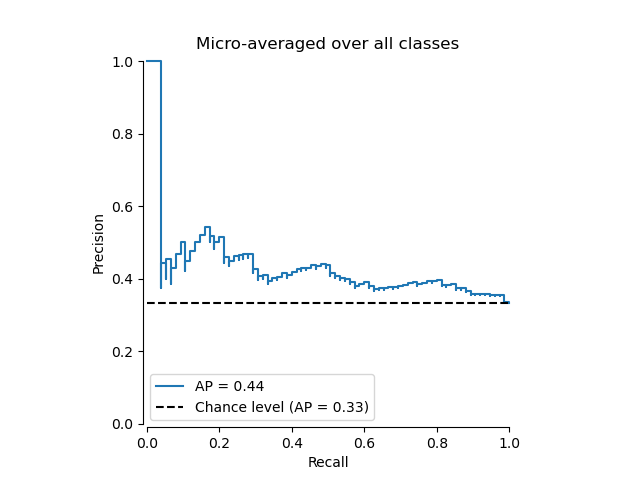
繪製微平均精確率-召回率曲線#
from collections import Counter

display = PrecisionRecallDisplay(
    recall=recall["micro"],
    precision=precision["micro"],
    average_precision=average_precision["micro"],
    prevalence_pos_label=Counter(Y_test.ravel())[1] / Y_test.size,
)
display.plot(plot_chance_level=True, despine=True)
_ = display.ax_.set_title("Micro-averaged over all classes")
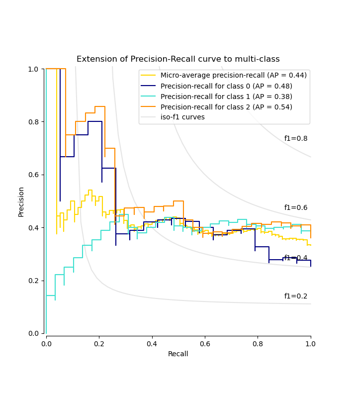
繪製每個類別的精確率-召回率曲線和等 f1 曲線#
from itertools import cycle

import matplotlib.pyplot as plt

# setup plot details
colors = cycle(["navy", "turquoise", "darkorange", "cornflowerblue", "teal"])

_, ax = plt.subplots(figsize=(7, 8))

f_scores = np.linspace(0.2, 0.8, num=4)
lines, labels = [], []
for f_score in f_scores:
    x = np.linspace(0.01, 1)
    y = f_score * x / (2 * x - f_score)
    (l,) = plt.plot(x[y >= 0], y[y >= 0], color="gray", alpha=0.2)
    plt.annotate("f1={0:0.1f}".format(f_score), xy=(0.9, y[45] + 0.02))

display = PrecisionRecallDisplay(
    recall=recall["micro"],
    precision=precision["micro"],
    average_precision=average_precision["micro"],
)
display.plot(ax=ax, name="Micro-average precision-recall", color="gold")

for i, color in zip(range(n_classes), colors):
    display = PrecisionRecallDisplay(
        recall=recall[i],
        precision=precision[i],
        average_precision=average_precision[i],
    )
    display.plot(
        ax=ax, name=f"Precision-recall for class {i}", color=color, despine=True
    )

# add the legend for the iso-f1 curves
handles, labels = display.ax_.get_legend_handles_labels()
handles.extend([l])
labels.extend(["iso-f1 curves"])
# set the legend and the axes
ax.legend(handles=handles, labels=labels, loc="best")
ax.set_title("Extension of Precision-Recall curve to multi-class")

plt.show()
腳本總執行時間:(0 分鐘 0.419 秒)
相關範例