注意
前往結尾以下載完整的範例程式碼。或透過 JupyterLite 或 Binder 在您的瀏覽器中執行此範例
基於模型和循序特徵選擇#
此範例說明並比較兩種特徵選擇方法:SelectFromModel 基於特徵重要性,以及 SequentialFeatureSelector 依賴貪婪方法。
我們使用糖尿病資料集,其中包含從 442 位糖尿病患者收集的 10 個特徵。
作者:Manoj Kumar、Maria Telenczuk、Nicolas Hug。
授權:BSD 3 條款
# Authors: The scikit-learn developers
# SPDX-License-Identifier: BSD-3-Clause
載入資料#
我們首先載入 scikit-learn 提供的糖尿病資料集,並印出其描述
from sklearn.datasets import load_diabetes

diabetes = load_diabetes()
X, y = diabetes.data, diabetes.target
print(diabetes.DESCR)
.. _diabetes_dataset:

Diabetes dataset
----------------

Ten baseline variables, age, sex, body mass index, average blood
pressure, and six blood serum measurements were obtained for each of n =
442 diabetes patients, as well as the response of interest, a
quantitative measure of disease progression one year after baseline.

**Data Set Characteristics:**

:Number of Instances: 442

:Number of Attributes: First 10 columns are numeric predictive values

:Target: Column 11 is a quantitative measure of disease progression one year after baseline

:Attribute Information:
    - age     age in years
    - sex
    - bmi     body mass index
    - bp      average blood pressure
    - s1      tc, total serum cholesterol
    - s2      ldl, low-density lipoproteins
    - s3      hdl, high-density lipoproteins
    - s4      tch, total cholesterol / HDL
    - s5      ltg, possibly log of serum triglycerides level
    - s6      glu, blood sugar level

Note: Each of these 10 feature variables have been mean centered and scaled by the standard deviation times the square root of `n_samples` (i.e. the sum of squares of each column totals 1).

Source URL:
https://www4.stat.ncsu.edu/~boos/var.select/diabetes.html

For more information see:
Bradley Efron, Trevor Hastie, Iain Johnstone and Robert Tibshirani (2004) "Least Angle Regression," Annals of Statistics (with discussion), 407-499.
(https://web.stanford.edu/~hastie/Papers/LARS/LeastAngle_2002.pdf)
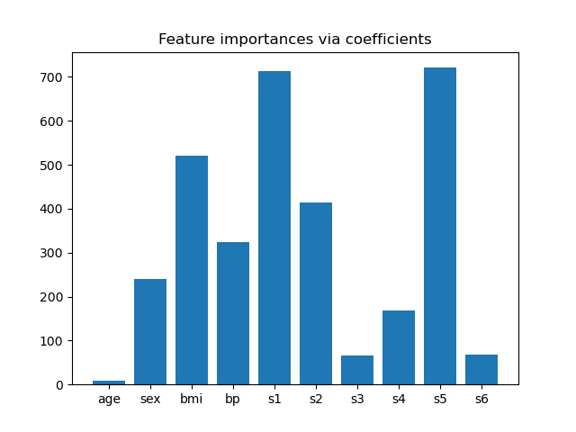
來自係數的特徵重要性#
為了了解特徵的重要性,我們將使用 RidgeCV 估算器。絕對 coef_ 值最高的特徵被認為是最重要的。我們可以觀察係數,而無需縮放它們 (或縮放資料),因為從上面的描述中,我們知道特徵已經過標準化。如需更完整地解釋線性模型的係數,您可以參考 線性模型係數解釋中常見的陷阱。# noqa: E501
import matplotlib.pyplot as plt
import numpy as np

from sklearn.linear_model import RidgeCV

ridge = RidgeCV(alphas=np.logspace(-6, 6, num=5)).fit(X, y)
importance = np.abs(ridge.coef_)
feature_names = np.array(diabetes.feature_names)
plt.bar(height=importance, x=feature_names)
plt.title("Feature importances via coefficients")
plt.show()
根據重要性選擇特徵#
現在我們想根據係數選擇最重要的兩個特徵。SelectFromModel 專為此目的而設計。SelectFromModel 接受 threshold 參數,並將選擇重要性 (由係數定義) 高於此閾值的特徵。
由於我們只想選擇 2 個特徵,我們將此閾值設定為略高於第三個最重要的特徵的係數。
from time import time

from sklearn.feature_selection import SelectFromModel

threshold = np.sort(importance)[-3] + 0.01

tic = time()
sfm = SelectFromModel(ridge, threshold=threshold).fit(X, y)
toc = time()
print(f"Features selected by SelectFromModel: {feature_names[sfm.get_support()]}")
print(f"Done in {toc - tic:.3f}s")
Features selected by SelectFromModel: ['s1' 's5']
Done in 0.002s
使用循序特徵選擇選擇特徵#
選擇特徵的另一種方法是使用 SequentialFeatureSelector (SFS)。SFS 是一種貪婪程序,在每次迭代中,我們都會根據交叉驗證分數選擇最佳的新特徵來添加到我們選擇的特徵中。也就是說,我們從 0 個特徵開始,並選擇得分最高的最佳單一特徵。重複此程序,直到我們達到所需數量的選擇特徵。
我們也可以朝相反的方向 (向後 SFS) 進行,即從所有特徵開始,並貪婪地選擇要逐一移除的特徵。我們在此處說明兩種方法。
from sklearn.feature_selection import SequentialFeatureSelector

tic_fwd = time()
sfs_forward = SequentialFeatureSelector(
    ridge, n_features_to_select=2, direction="forward"
).fit(X, y)
toc_fwd = time()

tic_bwd = time()
sfs_backward = SequentialFeatureSelector(
    ridge, n_features_to_select=2, direction="backward"
).fit(X, y)
toc_bwd = time()

print(
    "Features selected by forward sequential selection: "
    f"{feature_names[sfs_forward.get_support()]}"
)
print(f"Done in {toc_fwd - tic_fwd:.3f}s")
print(
    "Features selected by backward sequential selection: "
    f"{feature_names[sfs_backward.get_support()]}"
)
print(f"Done in {toc_bwd - tic_bwd:.3f}s")
Features selected by forward sequential selection: ['bmi' 's5']
Done in 0.245s
Features selected by backward sequential selection: ['bmi' 's5']
Done in 0.682s
有趣的是,向前和向後選擇選擇了相同的特徵集。一般而言,情況並非如此,這兩種方法會導致不同的結果。
我們還注意到,SFS 選擇的特徵與特徵重要性選擇的特徵不同:SFS 選擇 bmi 而不是 s1。不過,這聽起來很合理,因為根據係數,bmi 對應於第三個最重要的特徵。考慮到 SFS 完全沒有使用係數,這相當了不起。
最後,我們應該注意到 SelectFromModel 比 SFS 快得多。事實上,SelectFromModel 只需要擬合一次模型,而 SFS 在每次迭代都需要交叉驗證許多不同的模型。然而,SFS 可以與任何模型一起使用,而 SelectFromModel 則要求底層的估計器公開 coef_ 屬性或 feature_importances_ 屬性。前向 SFS 比後向 SFS 快,因為它只需要執行 n_features_to_select = 2 次迭代,而後向 SFS 需要執行 n_features - n_features_to_select = 8 次迭代。
使用負容差值#
可以使用 SequentialFeatureSelector,透過 direction="backward" 和 tol 的負值,來移除數據集中存在的特徵,並返回原始特徵的較小子集。
我們首先載入乳癌數據集,其中包含 30 個不同的特徵和 569 個樣本。
import numpy as np

from sklearn.datasets import load_breast_cancer

breast_cancer_data = load_breast_cancer()
X, y = breast_cancer_data.data, breast_cancer_data.target
feature_names = np.array(breast_cancer_data.feature_names)
print(breast_cancer_data.DESCR)
.. _breast_cancer_dataset:

Breast cancer wisconsin (diagnostic) dataset
--------------------------------------------

**Data Set Characteristics:**

:Number of Instances: 569

:Number of Attributes: 30 numeric, predictive attributes and the class

:Attribute Information:
    - radius (mean of distances from center to points on the perimeter)
    - texture (standard deviation of gray-scale values)
    - perimeter
    - area
    - smoothness (local variation in radius lengths)
    - compactness (perimeter^2 / area - 1.0)
    - concavity (severity of concave portions of the contour)
    - concave points (number of concave portions of the contour)
    - symmetry
    - fractal dimension ("coastline approximation" - 1)

    The mean, standard error, and "worst" or largest (mean of the three
    worst/largest values) of these features were computed for each image,
    resulting in 30 features.  For instance, field 0 is Mean Radius, field
    10 is Radius SE, field 20 is Worst Radius.

    - class:
            - WDBC-Malignant
            - WDBC-Benign

:Summary Statistics:

===================================== ====== ======
                                        Min    Max
===================================== ====== ======
radius (mean):                        6.981  28.11
texture (mean):                       9.71   39.28
perimeter (mean):                     43.79  188.5
area (mean):                          143.5  2501.0
smoothness (mean):                    0.053  0.163
compactness (mean):                   0.019  0.345
concavity (mean):                     0.0    0.427
concave points (mean):                0.0    0.201
symmetry (mean):                      0.106  0.304
fractal dimension (mean):             0.05   0.097
radius (standard error):              0.112  2.873
texture (standard error):             0.36   4.885
perimeter (standard error):           0.757  21.98
area (standard error):                6.802  542.2
smoothness (standard error):          0.002  0.031
compactness (standard error):         0.002  0.135
concavity (standard error):           0.0    0.396
concave points (standard error):      0.0    0.053
symmetry (standard error):            0.008  0.079
fractal dimension (standard error):   0.001  0.03
radius (worst):                       7.93   36.04
texture (worst):                      12.02  49.54
perimeter (worst):                    50.41  251.2
area (worst):                         185.2  4254.0
smoothness (worst):                   0.071  0.223
compactness (worst):                  0.027  1.058
concavity (worst):                    0.0    1.252
concave points (worst):               0.0    0.291
symmetry (worst):                     0.156  0.664
fractal dimension (worst):            0.055  0.208
===================================== ====== ======

:Missing Attribute Values: None

:Class Distribution: 212 - Malignant, 357 - Benign

:Creator:  Dr. William H. Wolberg, W. Nick Street, Olvi L. Mangasarian

:Donor: Nick Street

:Date: November, 1995

This is a copy of UCI ML Breast Cancer Wisconsin (Diagnostic) datasets.
https://goo.gl/U2Uwz2

Features are computed from a digitized image of a fine needle
aspirate (FNA) of a breast mass.  They describe
characteristics of the cell nuclei present in the image.

Separating plane described above was obtained using
Multisurface Method-Tree (MSM-T) [K. P. Bennett, "Decision Tree
Construction Via Linear Programming." Proceedings of the 4th
Midwest Artificial Intelligence and Cognitive Science Society,
pp. 97-101, 1992], a classification method which uses linear
programming to construct a decision tree.  Relevant features
were selected using an exhaustive search in the space of 1-4
features and 1-3 separating planes.

The actual linear program used to obtain the separating plane
in the 3-dimensional space is that described in:
[K. P. Bennett and O. L. Mangasarian: "Robust Linear
Programming Discrimination of Two Linearly Inseparable Sets",
Optimization Methods and Software 1, 1992, 23-34].

This database is also available through the UW CS ftp server:

ftp ftp.cs.wisc.edu
cd math-prog/cpo-dataset/machine-learn/WDBC/

.. dropdown:: References

  - W.N. Street, W.H. Wolberg and O.L. Mangasarian. Nuclear feature extraction
    for breast tumor diagnosis. IS&T/SPIE 1993 International Symposium on
    Electronic Imaging: Science and Technology, volume 1905, pages 861-870,
    San Jose, CA, 1993.
  - O.L. Mangasarian, W.N. Street and W.H. Wolberg. Breast cancer diagnosis and
    prognosis via linear programming. Operations Research, 43(4), pages 570-577,
    July-August 1995.
  - W.H. Wolberg, W.N. Street, and O.L. Mangasarian. Machine learning techniques
    to diagnose breast cancer from fine-needle aspirates. Cancer Letters 77 (1994)
    163-171.
我們將使用帶有 SequentialFeatureSelector 的 LogisticRegression 估計器來執行特徵選擇。
from sklearn.linear_model import LogisticRegression
from sklearn.metrics import roc_auc_score
from sklearn.pipeline import make_pipeline
from sklearn.preprocessing import StandardScaler

for tol in [-1e-2, -1e-3, -1e-4]:
    start = time()
    feature_selector = SequentialFeatureSelector(
        LogisticRegression(),
        n_features_to_select="auto",
        direction="backward",
        scoring="roc_auc",
        tol=tol,
        n_jobs=2,
    )
    model = make_pipeline(StandardScaler(), feature_selector, LogisticRegression())
    model.fit(X, y)
    end = time()
    print(f"\ntol: {tol}")
    print(f"Features selected: {feature_names[model[1].get_support()]}")
    print(f"ROC AUC score: {roc_auc_score(y, model.predict_proba(X)[:, 1]):.3f}")
    print(f"Done in {end - start:.3f}s")
tol: -0.01
Features selected: ['worst perimeter']
ROC AUC score: 0.975
Done in 11.825s

tol: -0.001
Features selected: ['radius error' 'fractal dimension error' 'worst texture'
 'worst perimeter' 'worst concave points']
ROC AUC score: 0.997
Done in 11.348s

tol: -0.0001
Features selected: ['mean compactness' 'mean concavity' 'mean concave points' 'radius error'
 'area error' 'concave points error' 'symmetry error'
 'fractal dimension error' 'worst texture' 'worst perimeter' 'worst area'
 'worst concave points' 'worst symmetry']
ROC AUC score: 0.998
Done in 9.782s
我們可以發現,隨著 tol 的負值接近零,所選擇的特徵數量趨於增加。隨著 tol 的值更接近零,特徵選擇所花費的時間也會減少。
腳本的總運行時間: (0 分鐘 33.996 秒)
相關範例