注意
前往結尾下載完整的範例程式碼。或透過 JupyterLite 或 Binder 在您的瀏覽器中執行此範例
使用稀疏特徵對文字文件進行分類#
這是一個範例,展示如何使用 scikit-learn 使用 詞袋方法依主題對文件進行分類。此範例使用 Tf-idf 加權的文件詞彙稀疏矩陣來編碼特徵,並示範各種可以有效處理稀疏矩陣的分類器。
對於透過非監督式學習方法進行文件分析,請參閱範例腳本 使用 k-means 對文字文件進行分群。
# Authors: The scikit-learn developers
# SPDX-License-Identifier: BSD-3-Clause
載入並向量化 20 個新聞群組文字資料集#
我們定義一個函數,從 20 個新聞群組文字資料集載入資料,該資料集包含大約 18,000 個新聞群組貼文,分為 20 個主題,分為兩個子集:一個用於訓練(或開發),另一個用於測試(或用於效能評估)。請注意,預設情況下,文字範例包含一些訊息中繼資料,例如 'headers'、'footers'(簽名)和 'quotes' 到其他貼文。fetch_20newsgroups 函數因此接受一個名為 remove 的參數,以嘗試剝離此類資訊,這會使分類問題「太容易」。這是使用既不完美也不標準的簡單啟發法來實現的,因此預設為停用。
from time import time

from sklearn.datasets import fetch_20newsgroups
from sklearn.feature_extraction.text import TfidfVectorizer

categories = [
    "alt.atheism",
    "talk.religion.misc",
    "comp.graphics",
    "sci.space",
]


def size_mb(docs):
    return sum(len(s.encode("utf-8")) for s in docs) / 1e6


def load_dataset(verbose=False, remove=()):
    """Load and vectorize the 20 newsgroups dataset."""

    data_train = fetch_20newsgroups(
        subset="train",
        categories=categories,
        shuffle=True,
        random_state=42,
        remove=remove,
    )

    data_test = fetch_20newsgroups(
        subset="test",
        categories=categories,
        shuffle=True,
        random_state=42,
        remove=remove,
    )

    # order of labels in `target_names` can be different from `categories`
    target_names = data_train.target_names

    # split target in a training set and a test set
    y_train, y_test = data_train.target, data_test.target

    # Extracting features from the training data using a sparse vectorizer
    t0 = time()
    vectorizer = TfidfVectorizer(
        sublinear_tf=True, max_df=0.5, min_df=5, stop_words="english"
    )
    X_train = vectorizer.fit_transform(data_train.data)
    duration_train = time() - t0

    # Extracting features from the test data using the same vectorizer
    t0 = time()
    X_test = vectorizer.transform(data_test.data)
    duration_test = time() - t0

    feature_names = vectorizer.get_feature_names_out()

    if verbose:
        # compute size of loaded data
        data_train_size_mb = size_mb(data_train.data)
        data_test_size_mb = size_mb(data_test.data)

        print(
            f"{len(data_train.data)} documents - "
            f"{data_train_size_mb:.2f}MB (training set)"
        )
        print(f"{len(data_test.data)} documents - {data_test_size_mb:.2f}MB (test set)")
        print(f"{len(target_names)} categories")
        print(
            f"vectorize training done in {duration_train:.3f}s "
            f"at {data_train_size_mb / duration_train:.3f}MB/s"
        )
        print(f"n_samples: {X_train.shape[0]}, n_features: {X_train.shape[1]}")
        print(
            f"vectorize testing done in {duration_test:.3f}s "
            f"at {data_test_size_mb / duration_test:.3f}MB/s"
        )
        print(f"n_samples: {X_test.shape[0]}, n_features: {X_test.shape[1]}")

    return X_train, X_test, y_train, y_test, feature_names, target_names
詞袋文件分類器的分析#
現在我們將訓練分類器兩次,一次針對包含中繼資料的文字範例,一次在剝離中繼資料之後。對於這兩種情況,我們將使用混淆矩陣分析測試集上的分類錯誤,並檢查定義訓練模型分類函數的係數。
不含中繼資料剝離的模型#
我們首先使用自訂函數 load_dataset 載入不含中繼資料剝離的資料。
X_train, X_test, y_train, y_test, feature_names, target_names = load_dataset(
    verbose=True
)
2034 documents - 3.98MB (training set)
1353 documents - 2.87MB (test set)
4 categories
vectorize training done in 0.392s at 10.157MB/s
n_samples: 2034, n_features: 7831
vectorize testing done in 0.240s at 11.926MB/s
n_samples: 1353, n_features: 7831
我們第一個模型是 RidgeClassifier 類別的實例。這是一個線性分類模型,它使用 {-1, 1} 編碼目標上的均方誤差,每個可能的類別一個。與 LogisticRegression 不同,RidgeClassifier 不提供機率預測(沒有 predict_proba 方法),但通常訓練速度更快。
from sklearn.linear_model import RidgeClassifier

clf = RidgeClassifier(tol=1e-2, solver="sparse_cg")
clf.fit(X_train, y_train)
pred = clf.predict(X_test)
我們繪製此分類器的混淆矩陣,以找出分類錯誤中是否存在模式。
import matplotlib.pyplot as plt

from sklearn.metrics import ConfusionMatrixDisplay

fig, ax = plt.subplots(figsize=(10, 5))
ConfusionMatrixDisplay.from_predictions(y_test, pred, ax=ax)
ax.xaxis.set_ticklabels(target_names)
ax.yaxis.set_ticklabels(target_names)
_ = ax.set_title(
    f"Confusion Matrix for {clf.__class__.__name__}\non the original documents"
)
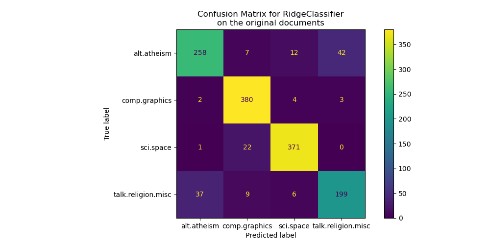
混淆矩陣突顯 alt.atheism 類別的文件經常與 talk.religion.misc 類別的文件混淆,反之亦然,這是預期的,因為這些主題在語義上是相關的。
我們也觀察到,sci.space 類別的某些文件可能會被錯誤分類為 comp.graphics,而相反的情況則較為罕見。需要手動檢查這些分類不佳的文件,以深入了解這種不對稱性。可能是太空主題的詞彙可能比電腦繪圖的詞彙更具體。
我們可以透過查看具有最高平均特徵影響的詞彙,更深入地了解此分類器如何做出決策
import numpy as np
import pandas as pd


def plot_feature_effects():
    # learned coefficients weighted by frequency of appearance
    average_feature_effects = clf.coef_ * np.asarray(X_train.mean(axis=0)).ravel()

    for i, label in enumerate(target_names):
        top5 = np.argsort(average_feature_effects[i])[-5:][::-1]
        if i == 0:
            top = pd.DataFrame(feature_names[top5], columns=[label])
            top_indices = top5
        else:
            top[label] = feature_names[top5]
            top_indices = np.concatenate((top_indices, top5), axis=None)
    top_indices = np.unique(top_indices)
    predictive_words = feature_names[top_indices]

    # plot feature effects
    bar_size = 0.25
    padding = 0.75
    y_locs = np.arange(len(top_indices)) * (4 * bar_size + padding)

    fig, ax = plt.subplots(figsize=(10, 8))
    for i, label in enumerate(target_names):
        ax.barh(
            y_locs + (i - 2) * bar_size,
            average_feature_effects[i, top_indices],
            height=bar_size,
            label=label,
        )
    ax.set(
        yticks=y_locs,
        yticklabels=predictive_words,
        ylim=[
            0 - 4 * bar_size,
            len(top_indices) * (4 * bar_size + padding) - 4 * bar_size,
        ],
    )
    ax.legend(loc="lower right")

    print("top 5 keywords per class:")
    print(top)

    return ax


_ = plot_feature_effects().set_title("Average feature effect on the original data")
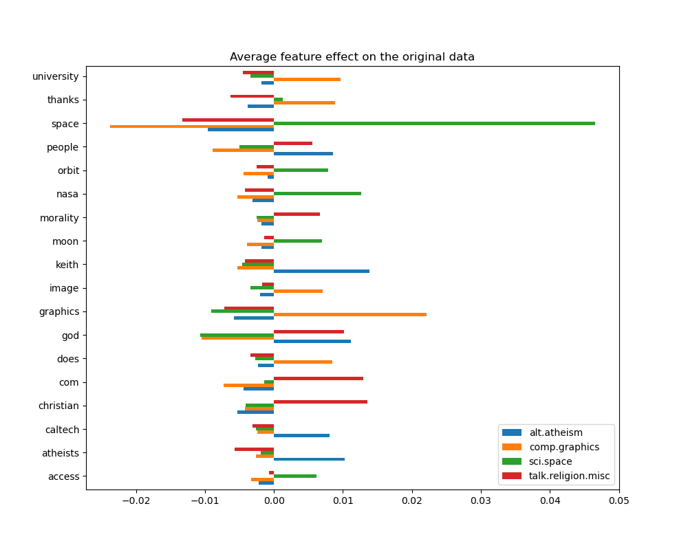
top 5 keywords per class:
  alt.atheism comp.graphics sci.space talk.religion.misc
0       keith      graphics     space          christian
1         god    university      nasa                com
2    atheists        thanks     orbit                god
3      people          does      moon           morality
4     caltech         image    access             people
我們可以觀察到,最具預測性的詞彙通常與單一類別強烈正相關,並與所有其他類別負相關。這些正相關性中的大多數都相當容易理解。但是,有些詞彙(例如 "god" 和 "people")與 "talk.misc.religion" 和 "alt.atheism" 都呈正相關,因為這兩個類別預期會共享一些共同的詞彙。但請注意,也有一些詞彙,例如 "christian" 和 "morality",僅與 "talk.misc.religion" 正相關。此外,在此版本的資料集中,由於資料集中來自某些中繼資料(例如電子郵件討論中先前電子郵件的寄件人電子郵件地址)的污染,"caltech" 一詞成為無神論最主要的預測特徵之一,如下所示
data_train = fetch_20newsgroups(
    subset="train", categories=categories, shuffle=True, random_state=42
)

for doc in data_train.data:
    if "caltech" in doc:
        print(doc)
        break
From: livesey@solntze.wpd.sgi.com (Jon Livesey)
Subject: Re: Morality? (was Re: <Political Atheists?)
Organization: sgi
Lines: 93
Distribution: world
NNTP-Posting-Host: solntze.wpd.sgi.com

In article <1qlettINN8oi@gap.caltech.edu>, keith@cco.caltech.edu (Keith Allan Schneider) writes:
|> livesey@solntze.wpd.sgi.com (Jon Livesey) writes:
|>
|> >>>Explain to me
|> >>>how instinctive acts can be moral acts, and I am happy to listen.
|> >>For example, if it were instinctive not to murder...
|> >
|> >Then not murdering would have no moral significance, since there
|> >would be nothing voluntary about it.
|>
|> See, there you go again, saying that a moral act is only significant
|> if it is "voluntary."  Why do you think this?

If you force me to do something, am I morally responsible for it?

|>
|> And anyway, humans have the ability to disregard some of their instincts.

Well, make up your mind.    Is it to be "instinctive not to murder"
or not?

|>
|> >>So, only intelligent beings can be moral, even if the bahavior of other
|> >>beings mimics theirs?
|> >
|> >You are starting to get the point.  Mimicry is not necessarily the
|> >same as the action being imitated.  A Parrot saying "Pretty Polly"
|> >isn't necessarily commenting on the pulchritude of Polly.
|>
|> You are attaching too many things to the term "moral," I think.
|> Let's try this:  is it "good" that animals of the same species
|> don't kill each other.  Or, do you think this is right?

It's not even correct.    Animals of the same species do kill
one another.

|>
|> Or do you think that animals are machines, and that nothing they do
|> is either right nor wrong?

Sigh.   I wonder how many times we have been round this loop.

I think that instinctive bahaviour has no moral significance.
I am quite prepared to believe that higher animals, such as
primates, have the beginnings of a moral sense, since they seem
to exhibit self-awareness.

|>
|>
|> >>Animals of the same species could kill each other arbitarily, but
|> >>they don't.
|> >
|> >They do.  I and other posters have given you many examples of exactly
|> >this, but you seem to have a very short memory.
|>
|> Those weren't arbitrary killings.  They were slayings related to some
|> sort of mating ritual or whatnot.

So what?     Are you trying to say that some killing in animals
has a moral significance and some does not?   Is this your
natural morality>


|>
|> >>Are you trying to say that this isn't an act of morality because
|> >>most animals aren't intelligent enough to think like we do?
|> >
|> >I'm saying:
|> >    "There must be the possibility that the organism - it's not
|> >    just people we are talking about - can consider alternatives."
|> >
|> >It's right there in the posting you are replying to.
|>
|> Yes it was, but I still don't understand your distinctions.  What
|> do you mean by "consider?"  Can a small child be moral?  How about
|> a gorilla?  A dolphin?  A platypus?  Where is the line drawn?  Does
|> the being need to be self aware?

Are you blind?   What do you think that this sentence means?

        "There must be the possibility that the organism - it's not
        just people we are talking about - can consider alternatives."

What would that imply?

|>
|> What *do* you call the mechanism which seems to prevent animals of
|> the same species from (arbitrarily) killing each other?  Don't
|> you find the fact that they don't at all significant?

I find the fact that they do to be significant.

jon.
此類標頭、簽名頁尾(以及先前訊息中引用的中繼資料)可以被視為人工洩漏新聞群組的附帶資訊,透過識別註冊的成員,我們寧願讓我們的文字分類器僅從每個文字文件的「主要內容」中學習,而不是依賴洩漏的作者身分。
含有中繼資料剝離的模型#
scikit-learn 中 20 個新聞群組資料集載入器的 remove 選項允許啟發式地嘗試篩除一些不必要的中繼資料,這會使分類問題變得更容易。請注意,此類文字內容的篩選遠非完美。
讓我們嘗試利用此選項來訓練一個文字分類器,該分類器不會過度依賴此類中繼資料來做出決策
(
    X_train,
    X_test,
    y_train,
    y_test,
    feature_names,
    target_names,
) = load_dataset(remove=("headers", "footers", "quotes"))

clf = RidgeClassifier(tol=1e-2, solver="sparse_cg")
clf.fit(X_train, y_train)
pred = clf.predict(X_test)

fig, ax = plt.subplots(figsize=(10, 5))
ConfusionMatrixDisplay.from_predictions(y_test, pred, ax=ax)
ax.xaxis.set_ticklabels(target_names)
ax.yaxis.set_ticklabels(target_names)
_ = ax.set_title(
    f"Confusion Matrix for {clf.__class__.__name__}\non filtered documents"
)
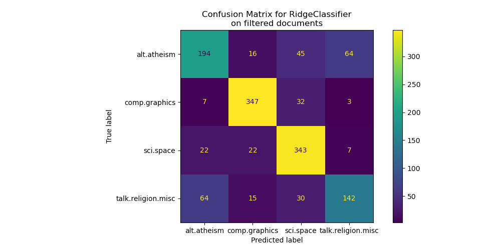
透過觀察混淆矩陣,可以更明顯地看出,使用元數據訓練的模型分數過於樂觀。在沒有元數據的情況下進行分類問題,其準確性較低,但更能代表預期的文本分類問題。
_ = plot_feature_effects().set_title("Average feature effects on filtered documents")
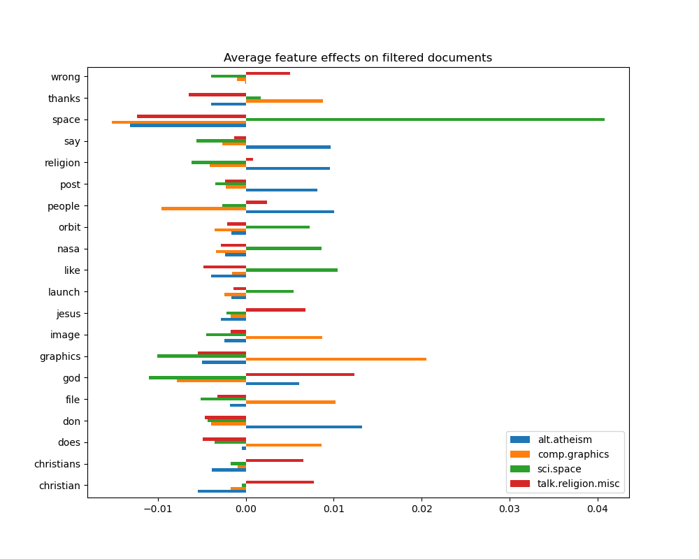
top 5 keywords per class:
  alt.atheism comp.graphics sci.space talk.religion.misc
0         don      graphics     space                god
1      people          file      like          christian
2         say        thanks      nasa              jesus
3    religion         image     orbit         christians
4        post          does    launch              wrong
在下一節中,我們將保留不含元數據的數據集,以比較幾種分類器。
分類器基準測試#
Scikit-learn 提供了許多不同種類的分類演算法。在本節中,我們將在相同的文本分類問題上訓練這些分類器的選擇,並測量它們的泛化效能(在測試集上的準確度)和計算效能(速度),包括訓練時間和測試時間。為此,我們定義了以下基準測試工具。
from sklearn import metrics
from sklearn.utils.extmath import density


def benchmark(clf, custom_name=False):
    print("_" * 80)
    print("Training: ")
    print(clf)
    t0 = time()
    clf.fit(X_train, y_train)
    train_time = time() - t0
    print(f"train time: {train_time:.3}s")

    t0 = time()
    pred = clf.predict(X_test)
    test_time = time() - t0
    print(f"test time:  {test_time:.3}s")

    score = metrics.accuracy_score(y_test, pred)
    print(f"accuracy:   {score:.3}")

    if hasattr(clf, "coef_"):
        print(f"dimensionality: {clf.coef_.shape[1]}")
        print(f"density: {density(clf.coef_)}")
        print()

    print()
    if custom_name:
        clf_descr = str(custom_name)
    else:
        clf_descr = clf.__class__.__name__
    return clf_descr, score, train_time, test_time
現在,我們使用 8 種不同的分類模型來訓練和測試數據集,並獲得每個模型的效能結果。本研究的目標是突顯針對此多類別文本分類問題,不同類型分類器的計算/準確度之間的權衡。
請注意,為了簡潔起見,這裡並未展示最重要的超參數值的調整過程,該過程是透過網格搜尋程序完成的。有關如何進行此類調整的演示,請參閱範例腳本文本特徵提取與評估的範例管道 # noqa: E501。
from sklearn.ensemble import RandomForestClassifier
from sklearn.linear_model import LogisticRegression, SGDClassifier
from sklearn.naive_bayes import ComplementNB
from sklearn.neighbors import KNeighborsClassifier, NearestCentroid
from sklearn.svm import LinearSVC

results = []
for clf, name in (
    (LogisticRegression(C=5, max_iter=1000), "Logistic Regression"),
    (RidgeClassifier(alpha=1.0, solver="sparse_cg"), "Ridge Classifier"),
    (KNeighborsClassifier(n_neighbors=100), "kNN"),
    (RandomForestClassifier(), "Random Forest"),
    # L2 penalty Linear SVC
    (LinearSVC(C=0.1, dual=False, max_iter=1000), "Linear SVC"),
    # L2 penalty Linear SGD
    (
        SGDClassifier(
            loss="log_loss", alpha=1e-4, n_iter_no_change=3, early_stopping=True
        ),
        "log-loss SGD",
    ),
    # NearestCentroid (aka Rocchio classifier)
    (NearestCentroid(), "NearestCentroid"),
    # Sparse naive Bayes classifier
    (ComplementNB(alpha=0.1), "Complement naive Bayes"),
):
    print("=" * 80)
    print(name)
    results.append(benchmark(clf, name))
================================================================================
Logistic Regression
________________________________________________________________________________
Training:
LogisticRegression(C=5, max_iter=1000)
train time: 0.177s
test time:  0.000734s
accuracy:   0.772
dimensionality: 5316
density: 1.0


================================================================================
Ridge Classifier
________________________________________________________________________________
Training:
RidgeClassifier(solver='sparse_cg')
train time: 0.0331s
test time:  0.000781s
accuracy:   0.76
dimensionality: 5316
density: 1.0


================================================================================
kNN
________________________________________________________________________________
Training:
KNeighborsClassifier(n_neighbors=100)
train time: 0.00105s
test time:  0.0734s
accuracy:   0.752

================================================================================
Random Forest
________________________________________________________________________________
Training:
RandomForestClassifier()
train time: 1.66s
test time:  0.0569s
accuracy:   0.704

================================================================================
Linear SVC
________________________________________________________________________________
Training:
LinearSVC(C=0.1, dual=False)
train time: 0.0293s
test time:  0.000699s
accuracy:   0.752
dimensionality: 5316
density: 1.0


================================================================================
log-loss SGD
________________________________________________________________________________
Training:
SGDClassifier(early_stopping=True, loss='log_loss', n_iter_no_change=3)
train time: 0.0311s
test time:  0.000672s
accuracy:   0.758
dimensionality: 5316
density: 1.0


================================================================================
NearestCentroid
________________________________________________________________________________
Training:
NearestCentroid()
train time: 0.187s
test time:  0.00177s
accuracy:   0.748

================================================================================
Complement naive Bayes
________________________________________________________________________________
Training:
ComplementNB(alpha=0.1)
train time: 0.00212s
test time:  0.000644s
accuracy:   0.779
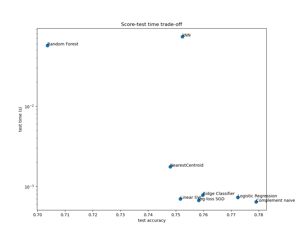
繪製每個分類器的準確度、訓練和測試時間圖#
散佈圖顯示了每個分類器的測試準確度與訓練和測試時間之間的權衡。
indices = np.arange(len(results))

results = [[x[i] for x in results] for i in range(4)]

clf_names, score, training_time, test_time = results
training_time = np.array(training_time)
test_time = np.array(test_time)

fig, ax1 = plt.subplots(figsize=(10, 8))
ax1.scatter(score, training_time, s=60)
ax1.set(
    title="Score-training time trade-off",
    yscale="log",
    xlabel="test accuracy",
    ylabel="training time (s)",
)
fig, ax2 = plt.subplots(figsize=(10, 8))
ax2.scatter(score, test_time, s=60)
ax2.set(
    title="Score-test time trade-off",
    yscale="log",
    xlabel="test accuracy",
    ylabel="test time (s)",
)

for i, txt in enumerate(clf_names):
    ax1.annotate(txt, (score[i], training_time[i]))
    ax2.annotate(txt, (score[i], test_time[i]))
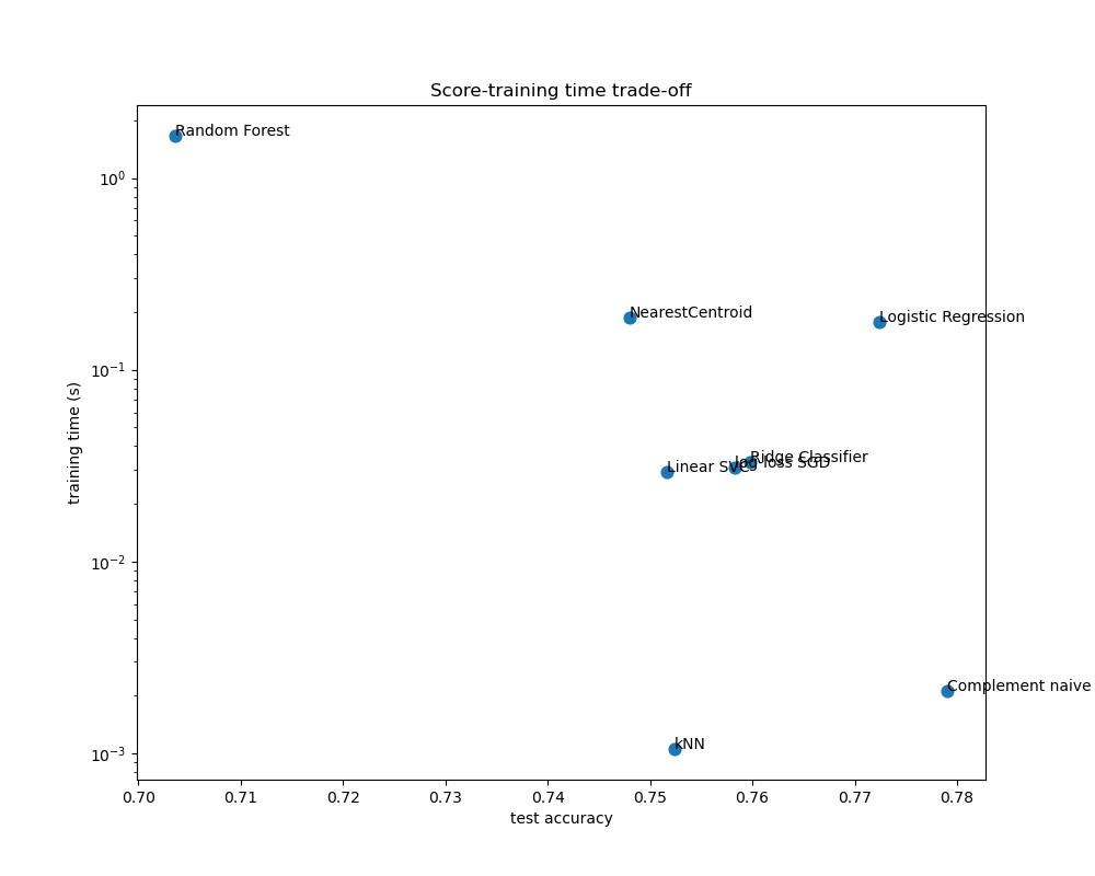
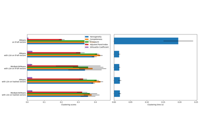
樸素貝葉斯模型在分數與訓練/測試時間之間具有最佳的權衡,而隨機森林的訓練速度慢、預測成本高,且準確度相對較差。這是預期的結果:對於高維度預測問題,線性模型通常更適合,因為當特徵空間具有 10,000 個或更多維度時,大多數問題都會變成線性可分的。
線性模型的訓練速度和準確度差異可以用它們優化的損失函數種類以及它們使用的正規化類型來解釋。請注意,某些具有相同損失但使用不同求解器或正規化配置的線性模型可能會產生不同的擬合時間和測試準確度。我們可以在第二張圖中觀察到,一旦經過訓練,所有線性模型都具有大致相同的預測速度,這是預期的,因為它們都實現了相同的預測函數。
KNeighborsClassifier 的準確度相對較低,且測試時間最長。預測時間長也是預期的:對於每次預測,模型都必須計算測試樣本與訓練集中每個文檔之間的成對距離,這在計算上非常昂貴。此外,「維度詛咒」損害了該模型在高維度文本分類問題的特徵空間中產生競爭性準確度的能力。
腳本總執行時間:(0 分鐘 6.776 秒)
相關範例