注意
前往結尾 以下載完整的範例程式碼。或透過 JupyterLite 或 Binder 在您的瀏覽器中執行此範例
Lasso 模型選擇:AIC-BIC / 交叉驗證#
此範例著重於 Lasso 模型的模型選擇,這些模型是具有用於迴歸問題的 L1 懲罰的線性模型。
實際上,可以使用幾種策略來選擇正規化參數的值:透過交叉驗證或使用資訊準則(即 AIC 或 BIC)。
在接下來的內容中,我們將詳細討論不同的策略。
# Authors: The scikit-learn developers
# SPDX-License-Identifier: BSD-3-Clause
資料集#
在本範例中,我們將使用糖尿病資料集。
from sklearn.datasets import load_diabetes

X, y = load_diabetes(return_X_y=True, as_frame=True)
X.head()
此外,我們將一些隨機特徵新增至原始資料,以更好地說明 Lasso 模型執行的特徵選擇。
import numpy as np
import pandas as pd

rng = np.random.RandomState(42)
n_random_features = 14
X_random = pd.DataFrame(
    rng.randn(X.shape[0], n_random_features),
    columns=[f"random_{i:02d}" for i in range(n_random_features)],
)
X = pd.concat([X, X_random], axis=1)
# Show only a subset of the columns
X[X.columns[::3]].head()
透過資訊準則選擇 Lasso#
LassoLarsIC 提供 Lasso 估算器,該估算器使用 Akaike 資訊準則 (AIC) 或貝氏資訊準則 (BIC) 來選擇正規化參數 alpha 的最佳值。
在擬合模型之前,我們將使用 StandardScaler 標準化資料。此外,我們將測量擬合和調整超參數 alpha 的時間,以便與交叉驗證策略進行比較。
我們將首先使用 AIC 準則擬合 Lasso 模型。
import time

from sklearn.linear_model import LassoLarsIC
from sklearn.pipeline import make_pipeline
from sklearn.preprocessing import StandardScaler

start_time = time.time()
lasso_lars_ic = make_pipeline(StandardScaler(), LassoLarsIC(criterion="aic")).fit(X, y)
fit_time = time.time() - start_time
我們儲存 fit 期間使用的每個 alpha 值的 AIC 度量。
results = pd.DataFrame(
    {
        "alphas": lasso_lars_ic[-1].alphas_,
        "AIC criterion": lasso_lars_ic[-1].criterion_,
    }
).set_index("alphas")
alpha_aic = lasso_lars_ic[-1].alpha_
現在,我們使用 BIC 準則執行相同的分析。
lasso_lars_ic.set_params(lassolarsic__criterion="bic").fit(X, y)
results["BIC criterion"] = lasso_lars_ic[-1].criterion_
alpha_bic = lasso_lars_ic[-1].alpha_
我們可以檢查哪個 alpha 值導致最小 AIC 和 BIC。
def highlight_min(x):
    x_min = x.min()
    return ["font-weight: bold" if v == x_min else "" for v in x]


results.style.apply(highlight_min)
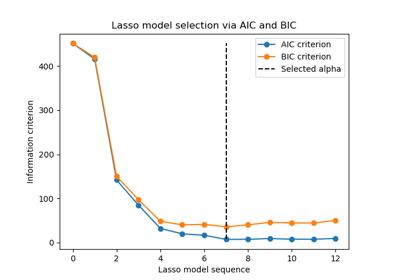
最後,我們可以繪製不同 alpha 值的 AIC 和 BIC 值。圖中的垂直線對應於為每個準則選擇的 alpha。選取的 alpha 對應於 AIC 或 BIC 準則的最小值。
ax = results.plot()
ax.vlines(
    alpha_aic,
    results["AIC criterion"].min(),
    results["AIC criterion"].max(),
    label="alpha: AIC estimate",
    linestyles="--",
    color="tab:blue",
)
ax.vlines(
    alpha_bic,
    results["BIC criterion"].min(),
    results["BIC criterion"].max(),
    label="alpha: BIC estimate",
    linestyle="--",
    color="tab:orange",
)
ax.set_xlabel(r"$\alpha$")
ax.set_ylabel("criterion")
ax.set_xscale("log")
ax.legend()
_ = ax.set_title(
    f"Information-criterion for model selection (training time {fit_time:.2f}s)"
)
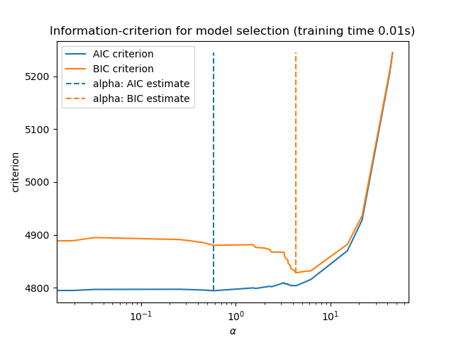
使用資訊準則的模型選擇非常快。它依賴於計算提供給 fit 的樣本內集合的準則。這兩個準則都根據訓練集錯誤估計模型泛化錯誤,並懲罰這種過於樂觀的錯誤。但是,此懲罰依賴於對自由度和雜訊變異數的正確估計。兩者都是針對大樣本 (漸近結果) 推導的,並假設模型是正確的,即資料實際上是由此模型產生的。
當問題條件不良時 (特徵多於樣本),這些模型也容易失效。然後,需要提供雜訊變異數的估計值。
透過交叉驗證選擇 Lasso#
Lasso 估算器可以使用不同的求解器來實作:座標下降和最小角度迴歸。它們在執行速度和數值錯誤的來源方面有所不同。
在 scikit-learn 中,有兩種不同的估算器可與整合交叉驗證一起使用:LassoCV 和 LassoLarsCV 分別使用座標下降和最小角度迴歸來解決問題。
在本節的其餘部分中,我們將介紹這兩種方法。對於這兩種演算法,我們將使用 20 折交叉驗證策略。
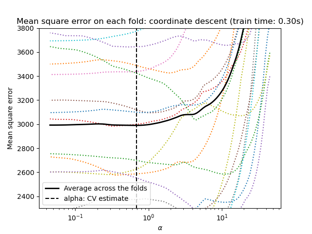
透過座標下降的 Lasso#
讓我們從使用 LassoCV 進行超參數調整開始。
from sklearn.linear_model import LassoCV

start_time = time.time()
model = make_pipeline(StandardScaler(), LassoCV(cv=20)).fit(X, y)
fit_time = time.time() - start_time
import matplotlib.pyplot as plt

ymin, ymax = 2300, 3800
lasso = model[-1]
plt.semilogx(lasso.alphas_, lasso.mse_path_, linestyle=":")
plt.plot(
    lasso.alphas_,
    lasso.mse_path_.mean(axis=-1),
    color="black",
    label="Average across the folds",
    linewidth=2,
)
plt.axvline(lasso.alpha_, linestyle="--", color="black", label="alpha: CV estimate")

plt.ylim(ymin, ymax)
plt.xlabel(r"$\alpha$")
plt.ylabel("Mean square error")
plt.legend()
_ = plt.title(
    f"Mean square error on each fold: coordinate descent (train time: {fit_time:.2f}s)"
)
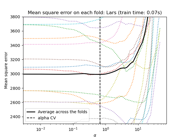
透過最小角度迴歸的 Lasso#
讓我們從使用 LassoLarsCV 進行超參數調整開始。
from sklearn.linear_model import LassoLarsCV

start_time = time.time()
model = make_pipeline(StandardScaler(), LassoLarsCV(cv=20)).fit(X, y)
fit_time = time.time() - start_time
lasso = model[-1]
plt.semilogx(lasso.cv_alphas_, lasso.mse_path_, ":")
plt.semilogx(
    lasso.cv_alphas_,
    lasso.mse_path_.mean(axis=-1),
    color="black",
    label="Average across the folds",
    linewidth=2,
)
plt.axvline(lasso.alpha_, linestyle="--", color="black", label="alpha CV")

plt.ylim(ymin, ymax)
plt.xlabel(r"$\alpha$")
plt.ylabel("Mean square error")
plt.legend()
_ = plt.title(f"Mean square error on each fold: Lars (train time: {fit_time:.2f}s)")
交叉驗證方法摘要#
這兩種演算法給出的結果大致相同。
Lars 僅針對路徑中的每個轉折計算解決方案路徑。因此,當轉折點很少時,它非常有效,如果特徵或樣本很少,則情況就是如此。此外,它可以在不設定任何超參數的情況下計算完整路徑。相反,座標下降會在預先指定的網格上計算路徑點(這裡我們使用預設值)。因此,如果網格點的數量小於路徑中的轉折點的數量,則它會更有效。如果特徵數量非常大,並且有足夠的樣本可以在每個交叉驗證折疊中選擇,那麼這樣的策略會很有趣。在數值誤差方面,對於高度相關的變數,Lars 會累積更多誤差,而座標下降演算法只會在網格上取樣路徑。
請注意,每個折疊的 alpha 的最佳值如何變化。這說明了為什麼當嘗試評估一種方法的效能時,巢狀交叉驗證是一種很好的策略,該方法的參數是透過交叉驗證選擇的:這種參數選擇對於僅在未見過的測試集上的最終評估可能不是最佳的。
結論#
在本教學中,我們介紹了兩種選擇最佳超參數 alpha 的方法:一種策略是僅使用訓練集和一些資訊準則來找到 alpha 的最佳值,另一種策略則是基於交叉驗證。
在這個例子中,兩種方法的工作方式相似。 樣本內超參數選擇甚至在計算效能方面顯示出其有效性。 然而,它只能在樣本數量相對於特徵數量足夠大時使用。
這就是為什麼通過交叉驗證進行超參數優化是一種安全的策略:它在不同的設定下都能工作。
腳本總執行時間: (0 分鐘 0.977 秒)
相關範例