使用隨機投影進行嵌入的 Johnson-Lindenstrauss 界限#

Johnson-Lindenstrauss 引理指出，任何高維資料集都可以隨機投影到較低維的歐幾里得空間，同時控制成對距離的失真。

# Authors: The scikit-learn developers
# SPDX-License-Identifier: BSD-3-Clause

import sys
from time import time

import matplotlib.pyplot as plt
import numpy as np

from sklearn.datasets import fetch_20newsgroups_vectorized, load_digits
from sklearn.metrics.pairwise import euclidean_distances
from sklearn.random_projection import (
    SparseRandomProjection,
    johnson_lindenstrauss_min_dim,
)

理論界限#

隨機投影 p 引入的失真由以下事實斷言：p 定義了一個具有良好機率的 eps 嵌入，定義如下

\[(1 - eps) \|u - v\|^2 < \|p(u) - p(v)\|^2 < (1 + eps) \|u - v\|^2\]

其中 u 和 v 是從形狀為 (n_samples, n_features) 的資料集中取得的任何列，而 p 是由形狀為 (n_components, n_features) 的隨機高斯 N(0, 1) 矩陣（或稀疏 Achlioptas 矩陣）進行的投影。

保證 eps 嵌入的最小元件數量由下式給出

\[n\_components \geq 4 log(n\_samples) / (eps^2 / 2 - eps^3 / 3)\]

第一個圖顯示，隨著樣本數 n_samples 的增加，為了保證 eps 嵌入，最小維度數 n_components 以對數方式增加。

# range of admissible distortions
eps_range = np.linspace(0.1, 0.99, 5)
colors = plt.cm.Blues(np.linspace(0.3, 1.0, len(eps_range)))

# range of number of samples (observation) to embed
n_samples_range = np.logspace(1, 9, 9)

plt.figure()
for eps, color in zip(eps_range, colors):
    min_n_components = johnson_lindenstrauss_min_dim(n_samples_range, eps=eps)
    plt.loglog(n_samples_range, min_n_components, color=color)

plt.legend([f"eps = {eps:0.1f}" for eps in eps_range], loc="lower right")
plt.xlabel("Number of observations to eps-embed")
plt.ylabel("Minimum number of dimensions")
plt.title("Johnson-Lindenstrauss bounds:\nn_samples vs n_components")
plt.show()

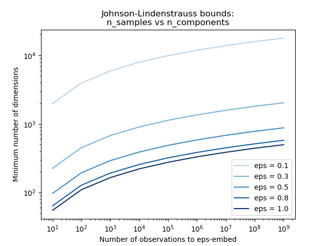
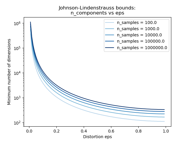
Johnson-Lindenstrauss bounds: n_samples vs n_components

第二個圖顯示，容許失真 eps 的增加允許大幅減少給定樣本數 n_samples 的最小維度數 n_components

# range of admissible distortions
eps_range = np.linspace(0.01, 0.99, 100)

# range of number of samples (observation) to embed
n_samples_range = np.logspace(2, 6, 5)
colors = plt.cm.Blues(np.linspace(0.3, 1.0, len(n_samples_range)))

plt.figure()
for n_samples, color in zip(n_samples_range, colors):
    min_n_components = johnson_lindenstrauss_min_dim(n_samples, eps=eps_range)
    plt.semilogy(eps_range, min_n_components, color=color)

plt.legend([f"n_samples = {n}" for n in n_samples_range], loc="upper right")
plt.xlabel("Distortion eps")
plt.ylabel("Minimum number of dimensions")
plt.title("Johnson-Lindenstrauss bounds:\nn_components vs eps")
plt.show()

Johnson-Lindenstrauss bounds: n_components vs eps

經驗驗證#

我們在 20 個新聞組文字文件（TF-IDF 字詞頻率）資料集或數字資料集上驗證上述界限

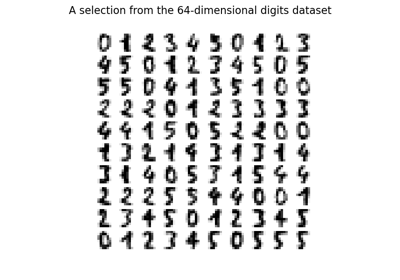
對於 20 個新聞組資料集，使用稀疏隨機矩陣將總共具有 10 萬個特徵的 300 個文件投影到較小的歐幾里得空間，目標維度數 n_components 的值各不相同。
對於數字資料集，將 300 個手寫數字圖片的 8x8 灰階像素資料隨機投影到維度數較大的空間，n_components 的值各不相同。

預設資料集是 20 個新聞組資料集。若要在數字資料集上執行此範例，請將 --use-digits-dataset 命令列引數傳遞給此指令碼。

if "--use-digits-dataset" in sys.argv:
    data = load_digits().data[:300]
else:
    data = fetch_20newsgroups_vectorized().data[:300]

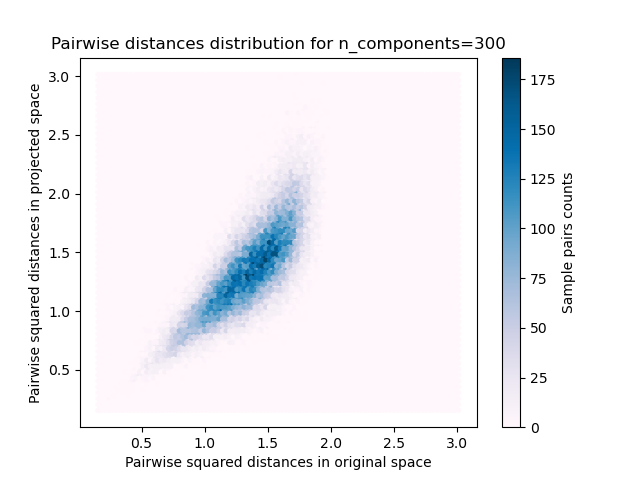
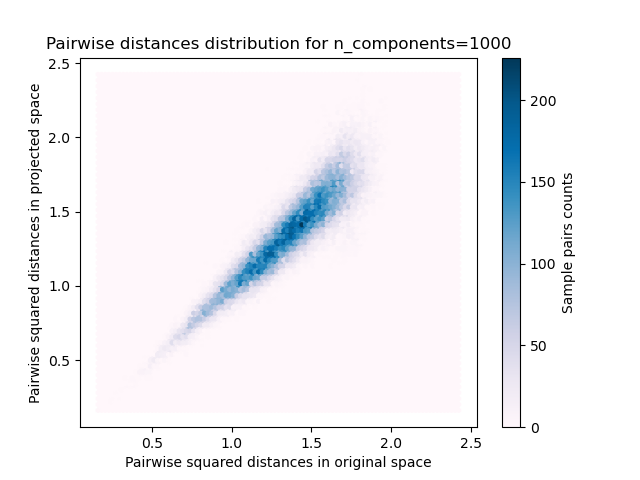
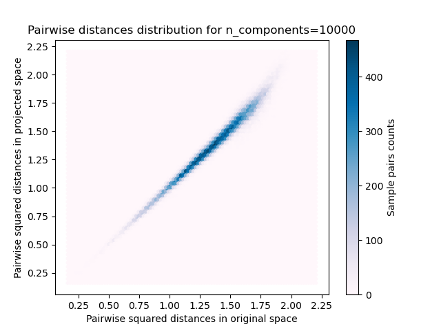
對於每個 n_components 值，我們繪製

樣本對的二維分佈，其中原始和投影空間中的成對距離分別作為 x 軸和 y 軸。
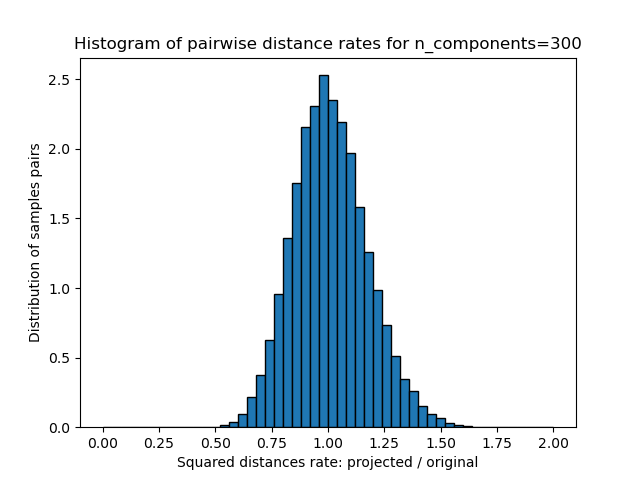
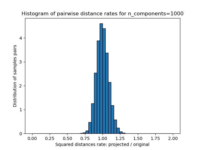
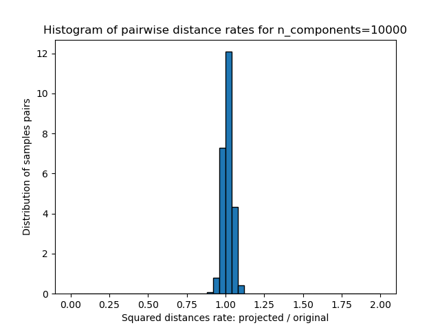
這些距離比率（投影/原始）的一維直方圖。

n_samples, n_features = data.shape
print(
    f"Embedding {n_samples} samples with dim {n_features} using various "
    "random projections"
)

n_components_range = np.array([300, 1_000, 10_000])
dists = euclidean_distances(data, squared=True).ravel()

# select only non-identical samples pairs
nonzero = dists != 0
dists = dists[nonzero]

for n_components in n_components_range:
    t0 = time()
    rp = SparseRandomProjection(n_components=n_components)
    projected_data = rp.fit_transform(data)
    print(
        f"Projected {n_samples} samples from {n_features} to {n_components} in "
        f"{time() - t0:0.3f}s"
    )
    if hasattr(rp, "components_"):
        n_bytes = rp.components_.data.nbytes
        n_bytes += rp.components_.indices.nbytes
        print(f"Random matrix with size: {n_bytes / 1e6:0.3f} MB")

    projected_dists = euclidean_distances(projected_data, squared=True).ravel()[nonzero]

    plt.figure()
    min_dist = min(projected_dists.min(), dists.min())
    max_dist = max(projected_dists.max(), dists.max())
    plt.hexbin(
        dists,
        projected_dists,
        gridsize=100,
        cmap=plt.cm.PuBu,
        extent=[min_dist, max_dist, min_dist, max_dist],
    )
    plt.xlabel("Pairwise squared distances in original space")
    plt.ylabel("Pairwise squared distances in projected space")
    plt.title("Pairwise distances distribution for n_components=%d" % n_components)
    cb = plt.colorbar()
    cb.set_label("Sample pairs counts")

    rates = projected_dists / dists
    print(f"Mean distances rate: {np.mean(rates):.2f} ({np.std(rates):.2f})")

    plt.figure()
    plt.hist(rates, bins=50, range=(0.0, 2.0), edgecolor="k", density=True)
    plt.xlabel("Squared distances rate: projected / original")
    plt.ylabel("Distribution of samples pairs")
    plt.title("Histogram of pairwise distance rates for n_components=%d" % n_components)

    # TODO: compute the expected value of eps and add them to the previous plot
    # as vertical lines / region

plt.show()

Embedding 300 samples with dim 130107 using various random projections
Projected 300 samples from 130107 to 300 in 0.296s
Random matrix with size: 1.293 MB
Mean distances rate: 1.01 (0.17)
Projected 300 samples from 130107 to 1000 in 1.039s
Random matrix with size: 4.323 MB
Mean distances rate: 1.00 (0.09)
Projected 300 samples from 130107 to 10000 in 8.094s
Random matrix with size: 43.268 MB
Mean distances rate: 1.01 (0.03)

我們可以看到，對於較小的 n_components 值，分佈範圍很廣，有許多失真的對，且分佈偏斜（由於左側距離總是正數的零比率硬限制），而對於較大的 n_components 值，失真受到控制，且距離透過隨機投影得到良好保留。