scikit-learn 0.22 的發布重點#

我們很高興宣佈發布 scikit-learn 0.22，其中包含許多錯誤修復和新功能！我們在下面詳細介紹此版本的一些主要功能。如需所有變更的完整清單，請參閱版本說明。

若要安裝最新版本 (使用 pip)

pip install --upgrade scikit-learn

或使用 conda

conda install -c conda-forge scikit-learn

# Authors: The scikit-learn developers
# SPDX-License-Identifier: BSD-3-Clause

新的繪圖 API#

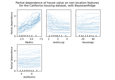
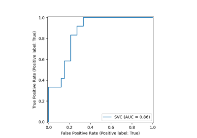
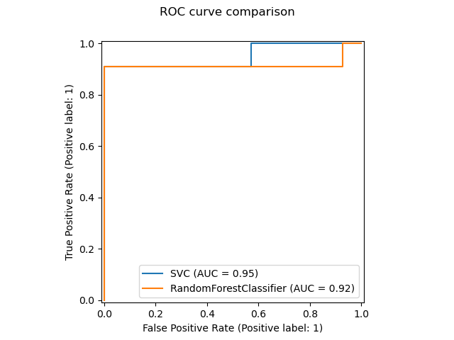
新的繪圖 API 可用於建立視覺化。這個新的 API 允許快速調整繪圖的視覺效果，而無需進行任何重新計算。也可以將不同的繪圖新增至同一個圖形。以下範例說明 plot_roc_curve，但其他繪圖實用工具也受到支援，例如 plot_partial_dependence、plot_precision_recall_curve 和 plot_confusion_matrix。請在使用者指南中閱讀有關此新 API 的更多資訊。

import matplotlib
import matplotlib.pyplot as plt

from sklearn.datasets import make_classification
from sklearn.ensemble import RandomForestClassifier

# from sklearn.metrics import plot_roc_curve
from sklearn.metrics import RocCurveDisplay
from sklearn.model_selection import train_test_split
from sklearn.svm import SVC
from sklearn.utils.fixes import parse_version

X, y = make_classification(random_state=0)
X_train, X_test, y_train, y_test = train_test_split(X, y, random_state=42)

svc = SVC(random_state=42)
svc.fit(X_train, y_train)
rfc = RandomForestClassifier(random_state=42)
rfc.fit(X_train, y_train)

# plot_roc_curve has been removed in version 1.2. From 1.2, use RocCurveDisplay instead.
# svc_disp = plot_roc_curve(svc, X_test, y_test)
# rfc_disp = plot_roc_curve(rfc, X_test, y_test, ax=svc_disp.ax_)
svc_disp = RocCurveDisplay.from_estimator(svc, X_test, y_test)
rfc_disp = RocCurveDisplay.from_estimator(rfc, X_test, y_test, ax=svc_disp.ax_)
rfc_disp.figure_.suptitle("ROC curve comparison")

plt.show()

堆疊分類器和迴歸器#

StackingClassifier和StackingRegressor允許您擁有一個包含最終分類器或迴歸器的估算器堆疊。堆疊泛化包括堆疊個別估算器的輸出，並使用分類器來計算最終預測。堆疊允許使用每個個別估算器的強度，方法是使用其輸出作為最終估算器的輸入。基本估算器在完整的 X 上進行擬合，而最終估算器則使用基本估算器的交叉驗證預測 (使用 cross_val_predict) 進行訓練。

請在使用者指南中閱讀更多資訊。

from sklearn.datasets import load_iris
from sklearn.ensemble import StackingClassifier
from sklearn.linear_model import LogisticRegression
from sklearn.model_selection import train_test_split
from sklearn.pipeline import make_pipeline
from sklearn.preprocessing import StandardScaler
from sklearn.svm import LinearSVC

X, y = load_iris(return_X_y=True)
estimators = [
    ("rf", RandomForestClassifier(n_estimators=10, random_state=42)),
    ("svr", make_pipeline(StandardScaler(), LinearSVC(dual="auto", random_state=42))),
]
clf = StackingClassifier(estimators=estimators, final_estimator=LogisticRegression())
X_train, X_test, y_train, y_test = train_test_split(X, y, stratify=y, random_state=42)
clf.fit(X_train, y_train).score(X_test, y_test)

0.9473684210526315

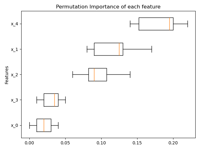
基於排列的特徵重要性#

inspection.permutation_importance 可用於取得任何擬合估算器之每個特徵重要性的估計值

import matplotlib.pyplot as plt
import numpy as np

from sklearn.datasets import make_classification
from sklearn.ensemble import RandomForestClassifier
from sklearn.inspection import permutation_importance

X, y = make_classification(random_state=0, n_features=5, n_informative=3)
feature_names = np.array([f"x_{i}" for i in range(X.shape[1])])

rf = RandomForestClassifier(random_state=0).fit(X, y)
result = permutation_importance(rf, X, y, n_repeats=10, random_state=0, n_jobs=2)

fig, ax = plt.subplots()
sorted_idx = result.importances_mean.argsort()

# `labels` argument in boxplot is deprecated in matplotlib 3.9 and has been
# renamed to `tick_labels`. The following code handles this, but as a
# scikit-learn user you probably can write simpler code by using `labels=...`
# (matplotlib < 3.9) or `tick_labels=...` (matplotlib >= 3.9).
tick_labels_parameter_name = (
    "tick_labels"
    if parse_version(matplotlib.__version__) >= parse_version("3.9")
    else "labels"
)
tick_labels_dict = {tick_labels_parameter_name: feature_names[sorted_idx]}
ax.boxplot(result.importances[sorted_idx].T, vert=False, **tick_labels_dict)
ax.set_title("Permutation Importance of each feature")
ax.set_ylabel("Features")
fig.tight_layout()
plt.show()

梯度提升的缺失值原生支援#

ensemble.HistGradientBoostingClassifier 和 ensemble.HistGradientBoostingRegressor 現在原生支援缺失值 (NaN)。這表示在訓練或預測時不需要填補資料。

from sklearn.ensemble import HistGradientBoostingClassifier

X = np.array([0, 1, 2, np.nan]).reshape(-1, 1)
y = [0, 0, 1, 1]

gbdt = HistGradientBoostingClassifier(min_samples_leaf=1).fit(X, y)
print(gbdt.predict(X))

[0 0 1 1]

預先計算的稀疏最近鄰圖#

大多數基於最近鄰圖的估算器現在都接受預先計算的稀疏圖作為輸入，以便為多個估算器擬合重複使用相同的圖。若要在管線中使用此功能，可以使用 memory 參數，以及兩個新的轉換器之一：neighbors.KNeighborsTransformer 和 neighbors.RadiusNeighborsTransformer。預先計算也可以由自訂估算器執行，以使用替代實作，例如近似最近鄰方法。請在使用者指南中查看更多詳細資訊。

from tempfile import TemporaryDirectory

from sklearn.manifold import Isomap
from sklearn.neighbors import KNeighborsTransformer
from sklearn.pipeline import make_pipeline

X, y = make_classification(random_state=0)

with TemporaryDirectory(prefix="sklearn_cache_") as tmpdir:
    estimator = make_pipeline(
        KNeighborsTransformer(n_neighbors=10, mode="distance"),
        Isomap(n_neighbors=10, metric="precomputed"),
        memory=tmpdir,
    )
    estimator.fit(X)

    # We can decrease the number of neighbors and the graph will not be
    # recomputed.
    estimator.set_params(isomap__n_neighbors=5)
    estimator.fit(X)

基於 KNN 的填補#

我們現在支援使用 k 最近鄰來填補缺失值。

每個樣本的缺失值會使用訓練集中 n_neighbors 個最近鄰居的平均值進行填補。如果兩個樣本的非缺失特徵彼此接近，則視為相近。預設情況下，會使用支援缺失值的歐幾里得距離度量 nan_euclidean_distances 來尋找最近鄰居。

請在使用者指南中閱讀更多資訊。

from sklearn.impute import KNNImputer

X = [[1, 2, np.nan], [3, 4, 3], [np.nan, 6, 5], [8, 8, 7]]
imputer = KNNImputer(n_neighbors=2)
print(imputer.fit_transform(X))

[[1.  2.  4. ]
 [3.  4.  3. ]
 [5.5 6.  5. ]
 [8.  8.  7. ]]

樹狀修剪#

現在可以在建立樹狀結構後修剪大多數基於樹狀結構的估計器。修剪是基於最小成本複雜性。請在使用者指南中閱讀更多詳細資訊。

X, y = make_classification(random_state=0)

rf = RandomForestClassifier(random_state=0, ccp_alpha=0).fit(X, y)
print(
    "Average number of nodes without pruning {:.1f}".format(
        np.mean([e.tree_.node_count for e in rf.estimators_])
    )
)

rf = RandomForestClassifier(random_state=0, ccp_alpha=0.05).fit(X, y)
print(
    "Average number of nodes with pruning {:.1f}".format(
        np.mean([e.tree_.node_count for e in rf.estimators_])
    )
)

Average number of nodes without pruning 22.3
Average number of nodes with pruning 6.4

從 OpenML 檢索資料框#

datasets.fetch_openml 現在可以回傳 pandas 資料框，從而正確處理具有異質資料的資料集。

from sklearn.datasets import fetch_openml

titanic = fetch_openml("titanic", version=1, as_frame=True, parser="pandas")
print(titanic.data.head()[["pclass", "embarked"]])

   pclass embarked
     1        S
     1        S
     1        S
     1        S
     1        S

檢查估計器的 scikit-learn 相容性#

開發人員可以使用 check_estimator 檢查其 scikit-learn 相容估計器的相容性。例如，check_estimator(LinearSVC()) 會通過檢查。

我們現在提供一個 pytest 專用的裝飾器，允許 pytest 獨立執行所有檢查，並報告失敗的檢查。

..note::: 此項目在 0.24 版本中略有更新，其中不再支援傳遞類別：請改為傳遞實例。

from sklearn.linear_model import LogisticRegression
from sklearn.tree import DecisionTreeRegressor
from sklearn.utils.estimator_checks import parametrize_with_checks


@parametrize_with_checks([LogisticRegression(), DecisionTreeRegressor()])
def test_sklearn_compatible_estimator(estimator, check):
    check(estimator)

ROC AUC 現在支援多類別分類#

roc_auc_score 函式也可以用於多類別分類。目前支援兩種平均策略：一對一演算法計算成對 ROC AUC 分數的平均值，而一對多演算法計算每個類別相對於所有其他類別的 ROC AUC 分數的平均值。在兩種情況下，多類別 ROC AUC 分數都是根據模型估計的樣本屬於特定類別的機率計算得出。OvO 和 OvR 演算法支援均勻加權 ( average='macro' ) 和按普及率加權 ( average='weighted' )。

請在使用者指南中閱讀更多資訊。

from sklearn.datasets import make_classification
from sklearn.metrics import roc_auc_score
from sklearn.svm import SVC

X, y = make_classification(n_classes=4, n_informative=16)
clf = SVC(decision_function_shape="ovo", probability=True).fit(X, y)
print(roc_auc_score(y, clf.predict_proba(X), multi_class="ovo"))