注意

前往末尾下載完整範例程式碼。或透過 JupyterLite 或 Binder 在您的瀏覽器中執行此範例

離群值偵測估算器的評估#

此範例比較兩種離群值偵測演算法，即局部離群值因子 (LOF) 和隔離森林 (IForest)，在 sklearn.datasets 中可用的真實世界資料集上。目的是顯示不同的演算法在不同的資料集上表現良好，並對比它們的訓練速度和對超參數的敏感度。

演算法在假設包含離群值的整個資料集上進行訓練 (沒有標籤)。

1. ROC 曲線是使用地面真值標籤的知識計算出來的，並使用 RocCurveDisplay 顯示。

效能以 ROC-AUC 來評估。

# Authors: The scikit-learn developers
# SPDX-License-Identifier: BSD-3-Clause

資料集預處理和模型訓練#

不同的離群值偵測模型需要不同的預處理。在存在類別變數的情況下，OrdinalEncoder 對於基於樹的模型 (例如 IsolationForest) 通常是一種很好的策略，而基於鄰居的模型 (例如 LocalOutlierFactor) 將受到序數編碼引起的排序的影響。為了避免產生排序，應該使用 OneHotEncoder。

基於鄰居的模型也可能需要縮放數值特徵 (請參閱例如重新調整對 k 近鄰模型的影響)。在存在離群值的情況下，一個好的選擇是使用 RobustScaler。

from sklearn.compose import ColumnTransformer
from sklearn.ensemble import IsolationForest
from sklearn.neighbors import LocalOutlierFactor
from sklearn.pipeline import make_pipeline
from sklearn.preprocessing import (
    OneHotEncoder,
    OrdinalEncoder,
    RobustScaler,
)


def make_estimator(name, categorical_columns=None, iforest_kw=None, lof_kw=None):
    """Create an outlier detection estimator based on its name."""
    if name == "LOF":
        outlier_detector = LocalOutlierFactor(**(lof_kw or {}))
        if categorical_columns is None:
            preprocessor = RobustScaler()
        else:
            preprocessor = ColumnTransformer(
                transformers=[("categorical", OneHotEncoder(), categorical_columns)],
                remainder=RobustScaler(),
            )
    else:  # name == "IForest"
        outlier_detector = IsolationForest(**(iforest_kw or {}))
        if categorical_columns is None:
            preprocessor = None
        else:
            ordinal_encoder = OrdinalEncoder(
                handle_unknown="use_encoded_value", unknown_value=-1
            )
            preprocessor = ColumnTransformer(
                transformers=[
                    ("categorical", ordinal_encoder, categorical_columns),
                ],
                remainder="passthrough",
            )

    return make_pipeline(preprocessor, outlier_detector)

以下 fit_predict 函式會傳回 X 的平均離群值分數。

from time import perf_counter


def fit_predict(estimator, X):
    tic = perf_counter()
    if estimator[-1].__class__.__name__ == "LocalOutlierFactor":
        estimator.fit(X)
        y_pred = estimator[-1].negative_outlier_factor_
    else:  # "IsolationForest"
        y_pred = estimator.fit(X).decision_function(X)
    toc = perf_counter()
    print(f"Duration for {model_name}: {toc - tic:.2f} s")
    return y_pred

在範例的其餘部分，我們每個區段處理一個資料集。在載入資料後，目標會被修改為由兩個類別組成：0 代表內圍值，1 代表離群值。由於 scikit-learn 文件計算的限制，某些資料集的樣本大小會使用分層 train_test_split 來縮減。

此外，我們設定 n_neighbors 以符合預期的異常數量 expected_n_anomalies = n_samples * expected_anomaly_fraction。這是一個很好的啟發式方法，只要離群值的比例不是非常低，原因在於 n_neighbors 應至少大於人口較少叢集中的樣本數 (請參閱使用局部離群值因子 (LOF) 進行離群值偵測)。

KDDCup99 - SA 資料集#

Kddcup 99 資料集是使用封閉網路和手動注入的攻擊產生的。SA 資料集是它的子集，其僅通過選擇所有正常資料和約 3% 的異常比例而獲得。

import numpy as np

from sklearn.datasets import fetch_kddcup99
from sklearn.model_selection import train_test_split

X, y = fetch_kddcup99(
    subset="SA", percent10=True, random_state=42, return_X_y=True, as_frame=True
)
y = (y != b"normal.").astype(np.int32)
X, _, y, _ = train_test_split(X, y, train_size=0.1, stratify=y, random_state=42)

n_samples, anomaly_frac = X.shape[0], y.mean()
print(f"{n_samples} datapoints with {y.sum()} anomalies ({anomaly_frac:.02%})")

10065 datapoints with 338 anomalies (3.36%)

SA 資料集包含 41 個特徵，其中 3 個是類別特徵：「protocol_type」、「service」和「flag」。

y_true = {}
y_pred = {"LOF": {}, "IForest": {}}
model_names = ["LOF", "IForest"]
cat_columns = ["protocol_type", "service", "flag"]

y_true["KDDCup99 - SA"] = y
for model_name in model_names:
    model = make_estimator(
        name=model_name,
        categorical_columns=cat_columns,
        lof_kw={"n_neighbors": int(n_samples * anomaly_frac)},
        iforest_kw={"random_state": 42},
    )
    y_pred[model_name]["KDDCup99 - SA"] = fit_predict(model, X)

Duration for LOF: 2.14 s
Duration for IForest: 0.31 s

森林覆蓋類型資料集#

森林覆蓋類型是一個多類別資料集，其中目標是給定一片森林中主要樹種。它包含 54 個特徵，其中一些特徵 (「Wilderness_Area」和「Soil_Type」) 已經以二進制編碼。雖然最初是作為分類任務，但可以將內圍值視為使用標籤 2 編碼的樣本，將離群值視為使用標籤 4 編碼的樣本。

from sklearn.datasets import fetch_covtype

X, y = fetch_covtype(return_X_y=True, as_frame=True)
s = (y == 2) + (y == 4)
X = X.loc[s]
y = y.loc[s]
y = (y != 2).astype(np.int32)

X, _, y, _ = train_test_split(X, y, train_size=0.05, stratify=y, random_state=42)
X_forestcover = X  # save X for later use

n_samples, anomaly_frac = X.shape[0], y.mean()
print(f"{n_samples} datapoints with {y.sum()} anomalies ({anomaly_frac:.02%})")

14302 datapoints with 137 anomalies (0.96%)

y_true["forestcover"] = y
for model_name in model_names:
    model = make_estimator(
        name=model_name,
        lof_kw={"n_neighbors": int(n_samples * anomaly_frac)},
        iforest_kw={"random_state": 42},
    )
    y_pred[model_name]["forestcover"] = fit_predict(model, X)

Duration for LOF: 1.89 s
Duration for IForest: 0.26 s

埃姆斯房屋資料集#

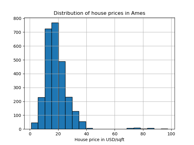
埃姆斯房屋資料集最初是一個迴歸資料集，其中目標是愛荷華州埃姆斯房屋的銷售價格。在這裡，我們將每平方英尺價格超過 70 美元的房屋視為離群值，從而將其轉換為離群值偵測問題。為了使問題更容易，我們刪除了每平方英尺價格在 40 美元到 70 美元之間的中間價格。

import matplotlib.pyplot as plt

from sklearn.datasets import fetch_openml

X, y = fetch_openml(name="ames_housing", version=1, return_X_y=True, as_frame=True)
y = y.div(X["Lot_Area"])

# None values in pandas 1.5.1 were mapped to np.nan in pandas 2.0.1
X["Misc_Feature"] = X["Misc_Feature"].cat.add_categories("NoInfo").fillna("NoInfo")
X["Mas_Vnr_Type"] = X["Mas_Vnr_Type"].cat.add_categories("NoInfo").fillna("NoInfo")

X.drop(columns="Lot_Area", inplace=True)
mask = (y < 40) | (y > 70)
X = X.loc[mask]
y = y.loc[mask]
y.hist(bins=20, edgecolor="black")
plt.xlabel("House price in USD/sqft")
_ = plt.title("Distribution of house prices in Ames")

y = (y > 70).astype(np.int32)

n_samples, anomaly_frac = X.shape[0], y.mean()
print(f"{n_samples} datapoints with {y.sum()} anomalies ({anomaly_frac:.02%})")

2714 datapoints with 30 anomalies (1.11%)

該資料集包含 46 個類別特徵。在這種情況下，使用 make_column_selector 來尋找它們比傳遞手動製作的列表更容易。

from sklearn.compose import make_column_selector as selector

categorical_columns_selector = selector(dtype_include="category")
cat_columns = categorical_columns_selector(X)

y_true["ames_housing"] = y
for model_name in model_names:
    model = make_estimator(
        name=model_name,
        categorical_columns=cat_columns,
        lof_kw={"n_neighbors": int(n_samples * anomaly_frac)},
        iforest_kw={"random_state": 42},
    )
    y_pred[model_name]["ames_housing"] = fit_predict(model, X)

Duration for LOF: 0.93 s
Duration for IForest: 0.24 s

心臟胎兒監護資料集#

「胎兒心電圖數據集」是一個多類別數據集，其中包含胎兒心電圖 (cardiotocograms)，類別以 1 到 10 的標籤編碼，代表胎兒心率 (FHR) 模式。在此，我們將第 3 類（少數類別）設定為代表離群值。它包含 30 個數值特徵，其中一些是二元編碼，另一些是連續的。

X, y = fetch_openml(name="cardiotocography", version=1, return_X_y=True, as_frame=False)
X_cardiotocography = X  # save X for later use
s = y == "3"
y = s.astype(np.int32)

n_samples, anomaly_frac = X.shape[0], y.mean()
print(f"{n_samples} datapoints with {y.sum()} anomalies ({anomaly_frac:.02%})")

2126 datapoints with 53 anomalies (2.49%)

y_true["cardiotocography"] = y
for model_name in model_names:
    model = make_estimator(
        name=model_name,
        lof_kw={"n_neighbors": int(n_samples * anomaly_frac)},
        iforest_kw={"random_state": 42},
    )
    y_pred[model_name]["cardiotocography"] = fit_predict(model, X)

Duration for LOF: 0.06 s
Duration for IForest: 0.16 s

繪製並解釋結果#

演算法的效能與偽陽性率 (FPR) 低時，真陽性率 (TPR) 有多好有關。最佳演算法在圖表的左上方有曲線，並且曲線下面積 (AUC) 接近 1。對角虛線代表離群值和正常值的隨機分類。

import math

from sklearn.metrics import RocCurveDisplay

cols = 2
pos_label = 0  # mean 0 belongs to positive class
datasets_names = y_true.keys()
rows = math.ceil(len(datasets_names) / cols)

fig, axs = plt.subplots(nrows=rows, ncols=cols, squeeze=False, figsize=(10, rows * 4))

for ax, dataset_name in zip(axs.ravel(), datasets_names):
    for model_idx, model_name in enumerate(model_names):
        display = RocCurveDisplay.from_predictions(
            y_true[dataset_name],
            y_pred[model_name][dataset_name],
            pos_label=pos_label,
            name=model_name,
            ax=ax,
            plot_chance_level=(model_idx == len(model_names) - 1),
            chance_level_kw={"linestyle": ":"},
        )
    ax.set_title(dataset_name)
_ = plt.tight_layout(pad=2.0)  # spacing between subplots

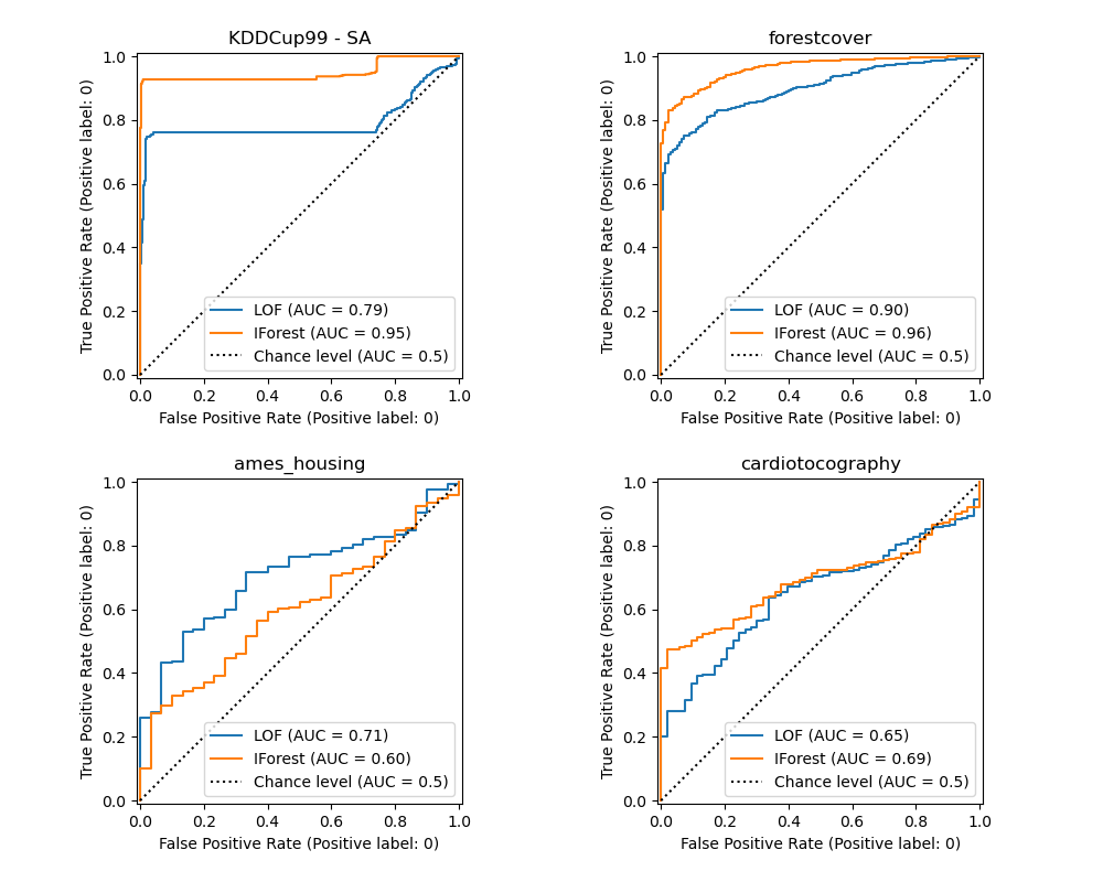
KDDCup99 - SA, forestcover, ames_housing, cardiotocography

我們觀察到，一旦調整了鄰居數量，對於森林覆蓋和胎兒心電圖數據集，LOF 和 IForest 在 ROC AUC 方面表現相似。對於 SA 數據集，IForest 的分數略好，而 LOF 在 Ames 房屋數據集上的表現明顯優於 IForest。

然而，請回想一下，在具有大量樣本的數據集上，Isolation Forest 的訓練速度往往比 LOF 快得多。LOF 需要計算成對距離以找到最近鄰居，其複雜度與觀察值的數量呈二次方關係。這可能使此方法在大數據集上難以使用。

消融研究#

在本節中，我們探討超參數 n_neighbors 以及縮放 LOF 模型數值變數的選擇所造成的影響。在這裡，我們使用「森林覆蓋類型」數據集，因為二元編碼的類別引入了 0 到 1 之間歐幾里得距離的自然尺度。然後，我們希望使用一種縮放方法來避免給予非二元特徵特權，並且該方法對於離群值足夠穩健，以至於尋找它們的任務不會變得太困難。

X = X_forestcover
y = y_true["forestcover"]

n_samples = X.shape[0]
n_neighbors_list = (n_samples * np.array([0.2, 0.02, 0.01, 0.001])).astype(np.int32)
model = make_pipeline(RobustScaler(), LocalOutlierFactor())

linestyles = ["solid", "dashed", "dashdot", ":", (5, (10, 3))]

fig, ax = plt.subplots()
for model_idx, (linestyle, n_neighbors) in enumerate(zip(linestyles, n_neighbors_list)):
    model.set_params(localoutlierfactor__n_neighbors=n_neighbors)
    model.fit(X)
    y_pred = model[-1].negative_outlier_factor_
    display = RocCurveDisplay.from_predictions(
        y,
        y_pred,
        pos_label=pos_label,
        name=f"n_neighbors = {n_neighbors}",
        ax=ax,
        plot_chance_level=(model_idx == len(n_neighbors_list) - 1),
        chance_level_kw={"linestyle": (0, (1, 10))},
        linestyle=linestyle,
        linewidth=2,
    )
_ = ax.set_title("RobustScaler with varying n_neighbors\non forestcover dataset")

RobustScaler with varying n_neighbors on forestcover dataset

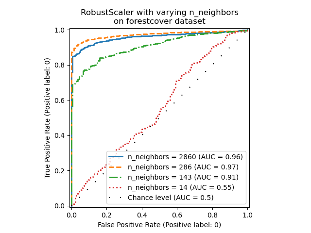
我們觀察到，鄰居數量對模型的效能有很大影響。如果可以存取（至少一些）真實標籤，則務必相應地調整 n_neighbors。一種方便的做法是探索 n_neighbors 的值，其數量級與預期的汙染程度相同。

from sklearn.preprocessing import MinMaxScaler, SplineTransformer, StandardScaler

preprocessor_list = [
    None,
    RobustScaler(),
    StandardScaler(),
    MinMaxScaler(),
    SplineTransformer(),
]
expected_anomaly_fraction = 0.02
lof = LocalOutlierFactor(n_neighbors=int(n_samples * expected_anomaly_fraction))

fig, ax = plt.subplots()
for model_idx, (linestyle, preprocessor) in enumerate(
    zip(linestyles, preprocessor_list)
):
    model = make_pipeline(preprocessor, lof)
    model.fit(X)
    y_pred = model[-1].negative_outlier_factor_
    display = RocCurveDisplay.from_predictions(
        y,
        y_pred,
        pos_label=pos_label,
        name=str(preprocessor).split("(")[0],
        ax=ax,
        plot_chance_level=(model_idx == len(preprocessor_list) - 1),
        chance_level_kw={"linestyle": (0, (1, 10))},
        linestyle=linestyle,
        linewidth=2,
    )
_ = ax.set_title("Fixed n_neighbors with varying preprocessing\non forestcover dataset")

Fixed n_neighbors with varying preprocessing on forestcover dataset

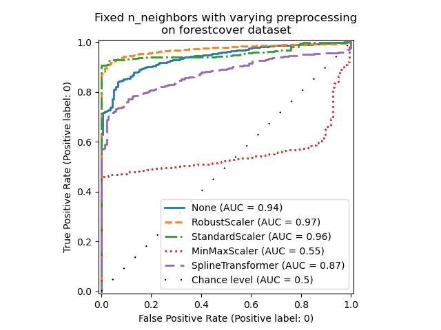
一方面，「RobustScaler」預設使用四分位數間距 (IQR) 來獨立縮放每個特徵，即資料的第 25 個和第 75 個百分位數之間的範圍。它通過減去中位數來中心化資料，然後通過除以 IQR 來縮放資料。IQR 對離群值具有穩健性：與範圍、平均值和標準差相比，中位數和四分位數間距受極端值的影響較小。此外，「RobustScaler」不像「StandardScaler」那樣擠壓邊緣離群值。

另一方面，「MinMaxScaler」會個別縮放每個特徵，使其範圍對應到零和一之間的範圍。如果資料中存在離群值，它們可能會將資料向最小值或最大值傾斜，導致具有較大邊緣離群值的資料分佈完全不同：所有非離群值可能因此幾乎被壓縮在一起。

我們還評估了完全不進行預處理（通過將 None 傳遞到管線中），「StandardScaler」和「SplineTransformer」。請參閱它們各自的文件以了解更多詳細資訊。

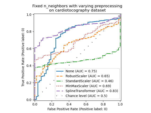
請注意，如下所示，最佳預處理取決於數據集

X = X_cardiotocography
y = y_true["cardiotocography"]

n_samples, expected_anomaly_fraction = X.shape[0], 0.025
lof = LocalOutlierFactor(n_neighbors=int(n_samples * expected_anomaly_fraction))

fig, ax = plt.subplots()
for model_idx, (linestyle, preprocessor) in enumerate(
    zip(linestyles, preprocessor_list)
):
    model = make_pipeline(preprocessor, lof)
    model.fit(X)
    y_pred = model[-1].negative_outlier_factor_
    display = RocCurveDisplay.from_predictions(
        y,
        y_pred,
        pos_label=pos_label,
        name=str(preprocessor).split("(")[0],
        ax=ax,
        plot_chance_level=(model_idx == len(preprocessor_list) - 1),
        chance_level_kw={"linestyle": (0, (1, 10))},
        linestyle=linestyle,
        linewidth=2,
    )
ax.set_title(
    "Fixed n_neighbors with varying preprocessing\non cardiotocography dataset"
)
plt.show()