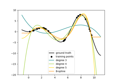
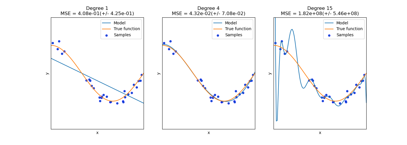
欠擬合 vs. 過擬合#

此範例示範了欠擬合和過擬合的問題，以及如何使用多項式特徵的線性迴歸來近似非線性函數。該圖顯示了我們要近似的函數，它是餘弦函數的一部分。此外，還顯示了真實函數的樣本和不同模型的近似值。這些模型具有不同次數的多項式特徵。我們可以看見，線性函數（1 次多項式）不足以擬合訓練樣本。這稱為欠擬合。 4 次多項式幾乎完美地近似真實函數。但是，對於更高的次數，模型將會過擬合訓練資料，即學習訓練資料的雜訊。我們使用交叉驗證來定量評估過擬合/欠擬合。我們計算驗證集上的均方誤差 (MSE)，值越高，模型從訓練資料中正確泛化的可能性就越低。

Degree 1 MSE = 4.08e-01(+/- 4.25e-01), Degree 4 MSE = 4.32e-02(+/- 7.08e-02), Degree 15 MSE = 1.82e+08(+/- 5.46e+08)

# Authors: The scikit-learn developers
# SPDX-License-Identifier: BSD-3-Clause

import matplotlib.pyplot as plt
import numpy as np

from sklearn.linear_model import LinearRegression
from sklearn.model_selection import cross_val_score
from sklearn.pipeline import Pipeline
from sklearn.preprocessing import PolynomialFeatures


def true_fun(X):
    return np.cos(1.5 * np.pi * X)


np.random.seed(0)

n_samples = 30
degrees = [1, 4, 15]

X = np.sort(np.random.rand(n_samples))
y = true_fun(X) + np.random.randn(n_samples) * 0.1

plt.figure(figsize=(14, 5))
for i in range(len(degrees)):
    ax = plt.subplot(1, len(degrees), i + 1)
    plt.setp(ax, xticks=(), yticks=())

    polynomial_features = PolynomialFeatures(degree=degrees[i], include_bias=False)
    linear_regression = LinearRegression()
    pipeline = Pipeline(
        [
            ("polynomial_features", polynomial_features),
            ("linear_regression", linear_regression),
        ]
    )
    pipeline.fit(X[:, np.newaxis], y)

    # Evaluate the models using crossvalidation
    scores = cross_val_score(
        pipeline, X[:, np.newaxis], y, scoring="neg_mean_squared_error", cv=10
    )

    X_test = np.linspace(0, 1, 100)
    plt.plot(X_test, pipeline.predict(X_test[:, np.newaxis]), label="Model")
    plt.plot(X_test, true_fun(X_test), label="True function")
    plt.scatter(X, y, edgecolor="b", s=20, label="Samples")
    plt.xlabel("x")
    plt.ylabel("y")
    plt.xlim((0, 1))
    plt.ylim((-2, 2))
    plt.legend(loc="best")
    plt.title(
        "Degree {}\nMSE = {:.2e}(+/- {:.2e})".format(
            degrees[i], -scores.mean(), scores.std()
        )
    )
plt.show()