注意
前往結尾以下載完整的範例程式碼。或透過 JupyterLite 或 Binder 在您的瀏覽器中執行此範例
模型複雜度影響#
展示模型複雜度如何影響預測準確性和計算效能。
- 我們將使用兩個資料集
糖尿病資料集用於迴歸。此資料集包含從糖尿病患者取得的 10 項測量值。任務是預測疾病進展;
20 個新聞群組文字資料集用於分類。此資料集包含新聞群組文章。任務是預測該文章是關於哪個主題(20 個主題中的一個)。
- 我們將在三個不同的估算器上建立複雜度影響模型
SGDClassifier(用於分類資料),實作隨機梯度下降學習;NuSVR(用於迴歸資料),實作 Nu 支援向量迴歸;GradientBoostingRegressor以前向階段方式建立加法模型。請注意,從中間資料集 (n_samples >= 10_000) 開始,HistGradientBoostingRegressor比GradientBoostingRegressor快得多,但此範例並非如此。
我們透過選擇每個選定模型中的相關模型參數,使模型複雜度發生變化。接下來,我們將測量對計算效能(延遲)和預測能力(MSE 或漢明損失)的影響。
# Authors: The scikit-learn developers
# SPDX-License-Identifier: BSD-3-Clause

import time

import matplotlib.pyplot as plt
import numpy as np

from sklearn import datasets
from sklearn.ensemble import GradientBoostingRegressor
from sklearn.linear_model import SGDClassifier
from sklearn.metrics import hamming_loss, mean_squared_error
from sklearn.model_selection import train_test_split
from sklearn.svm import NuSVR

# Initialize random generator
np.random.seed(0)
載入資料#
首先,我們載入這兩個資料集。
注意
我們使用 fetch_20newsgroups_vectorized 來下載 20 個新聞群組資料集。它會傳回可直接使用的特徵。
注意
20 個新聞群組資料集的 X 是稀疏矩陣,而糖尿病資料集的 X 則是 numpy 陣列。
def generate_data(case):
    """Generate regression/classification data."""
    if case == "regression":
        X, y = datasets.load_diabetes(return_X_y=True)
        train_size = 0.8
    elif case == "classification":
        X, y = datasets.fetch_20newsgroups_vectorized(subset="all", return_X_y=True)
        train_size = 0.4  # to make the example run faster

    X_train, X_test, y_train, y_test = train_test_split(
        X, y, train_size=train_size, random_state=0
    )

    data = {"X_train": X_train, "X_test": X_test, "y_train": y_train, "y_test": y_test}
    return data


regression_data = generate_data("regression")
classification_data = generate_data("classification")
基準影響#
接下來,我們可以計算參數對指定估算器的影響。在每一輪中,我們將以新的 changing_param 值設定估算器,並且我們將收集預測時間、預測效能和複雜度,以了解這些變更如何影響估算器。我們將使用作為參數傳遞的 complexity_computer 計算複雜度。
def benchmark_influence(conf):
    """
    Benchmark influence of `changing_param` on both MSE and latency.
    """
    prediction_times = []
    prediction_powers = []
    complexities = []
    for param_value in conf["changing_param_values"]:
        conf["tuned_params"][conf["changing_param"]] = param_value
        estimator = conf["estimator"](**conf["tuned_params"])

        print("Benchmarking %s" % estimator)
        estimator.fit(conf["data"]["X_train"], conf["data"]["y_train"])
        conf["postfit_hook"](estimator)
        complexity = conf["complexity_computer"](estimator)
        complexities.append(complexity)
        start_time = time.time()
        for _ in range(conf["n_samples"]):
            y_pred = estimator.predict(conf["data"]["X_test"])
        elapsed_time = (time.time() - start_time) / float(conf["n_samples"])
        prediction_times.append(elapsed_time)
        pred_score = conf["prediction_performance_computer"](
            conf["data"]["y_test"], y_pred
        )
        prediction_powers.append(pred_score)
        print(
            "Complexity: %d | %s: %.4f | Pred. Time: %fs\n"
            % (
                complexity,
                conf["prediction_performance_label"],
                pred_score,
                elapsed_time,
            )
        )
    return prediction_powers, prediction_times, complexities
選擇參數#
我們透過建立具有所有必要值的字典來選擇每個估算器的參數。changing_param 是每個估算器中會變動的參數名稱。複雜度將由 complexity_label 定義,並使用 complexity_computer 計算。另請注意,根據估算器類型,我們正在傳遞不同的資料。
def _count_nonzero_coefficients(estimator):
    a = estimator.coef_.toarray()
    return np.count_nonzero(a)


configurations = [
    {
        "estimator": SGDClassifier,
        "tuned_params": {
            "penalty": "elasticnet",
            "alpha": 0.001,
            "loss": "modified_huber",
            "fit_intercept": True,
            "tol": 1e-1,
            "n_iter_no_change": 2,
        },
        "changing_param": "l1_ratio",
        "changing_param_values": [0.25, 0.5, 0.75, 0.9],
        "complexity_label": "non_zero coefficients",
        "complexity_computer": _count_nonzero_coefficients,
        "prediction_performance_computer": hamming_loss,
        "prediction_performance_label": "Hamming Loss (Misclassification Ratio)",
        "postfit_hook": lambda x: x.sparsify(),
        "data": classification_data,
        "n_samples": 5,
    },
    {
        "estimator": NuSVR,
        "tuned_params": {"C": 1e3, "gamma": 2**-15},
        "changing_param": "nu",
        "changing_param_values": [0.05, 0.1, 0.2, 0.35, 0.5],
        "complexity_label": "n_support_vectors",
        "complexity_computer": lambda x: len(x.support_vectors_),
        "data": regression_data,
        "postfit_hook": lambda x: x,
        "prediction_performance_computer": mean_squared_error,
        "prediction_performance_label": "MSE",
        "n_samples": 15,
    },
    {
        "estimator": GradientBoostingRegressor,
        "tuned_params": {
            "loss": "squared_error",
            "learning_rate": 0.05,
            "max_depth": 2,
        },
        "changing_param": "n_estimators",
        "changing_param_values": [10, 25, 50, 75, 100],
        "complexity_label": "n_trees",
        "complexity_computer": lambda x: x.n_estimators,
        "data": regression_data,
        "postfit_hook": lambda x: x,
        "prediction_performance_computer": mean_squared_error,
        "prediction_performance_label": "MSE",
        "n_samples": 15,
    },
]
執行程式碼並繪製結果#
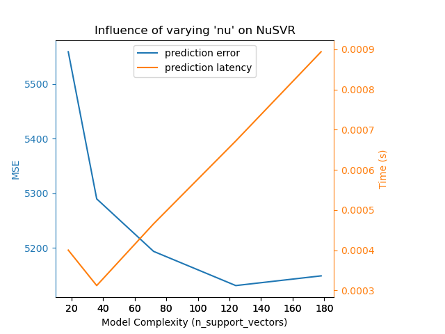
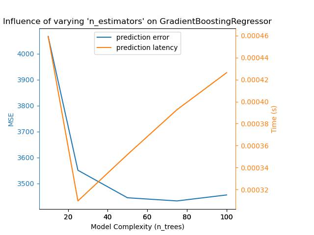
我們定義了執行基準測試所需的所有函式。現在,我們將迴圈處理先前定義的不同組態。隨後,我們可以分析從基準測試獲得的圖表:放寬 SGD 分類器中的 L1 懲罰會減少預測錯誤,但會導致訓練時間增加。我們可以針對訓練時間得出類似的分析,訓練時間會隨著 Nu-SVR 的支援向量數量而增加。然而,我們觀察到存在一個最佳的支援向量數量,可以減少預測錯誤。事實上,太少的支援向量會導致模型欠擬合,而太多的支援向量會導致模型過擬合。對於梯度提升模型,可以得出完全相同的結論。與 Nu-SVR 唯一不同之處在於,在集合中加入過多的樹木並不會造成損害。
def plot_influence(conf, mse_values, prediction_times, complexities):
    """
    Plot influence of model complexity on both accuracy and latency.
    """

    fig = plt.figure()
    fig.subplots_adjust(right=0.75)

    # first axes (prediction error)
    ax1 = fig.add_subplot(111)
    line1 = ax1.plot(complexities, mse_values, c="tab:blue", ls="-")[0]
    ax1.set_xlabel("Model Complexity (%s)" % conf["complexity_label"])
    y1_label = conf["prediction_performance_label"]
    ax1.set_ylabel(y1_label)

    ax1.spines["left"].set_color(line1.get_color())
    ax1.yaxis.label.set_color(line1.get_color())
    ax1.tick_params(axis="y", colors=line1.get_color())

    # second axes (latency)
    ax2 = fig.add_subplot(111, sharex=ax1, frameon=False)
    line2 = ax2.plot(complexities, prediction_times, c="tab:orange", ls="-")[0]
    ax2.yaxis.tick_right()
    ax2.yaxis.set_label_position("right")
    y2_label = "Time (s)"
    ax2.set_ylabel(y2_label)
    ax1.spines["right"].set_color(line2.get_color())
    ax2.yaxis.label.set_color(line2.get_color())
    ax2.tick_params(axis="y", colors=line2.get_color())

    plt.legend(
        (line1, line2), ("prediction error", "prediction latency"), loc="upper center"
    )

    plt.title(
        "Influence of varying '%s' on %s"
        % (conf["changing_param"], conf["estimator"].__name__)
    )


for conf in configurations:
    prediction_performances, prediction_times, complexities = benchmark_influence(conf)
    plot_influence(conf, prediction_performances, prediction_times, complexities)
plt.show()
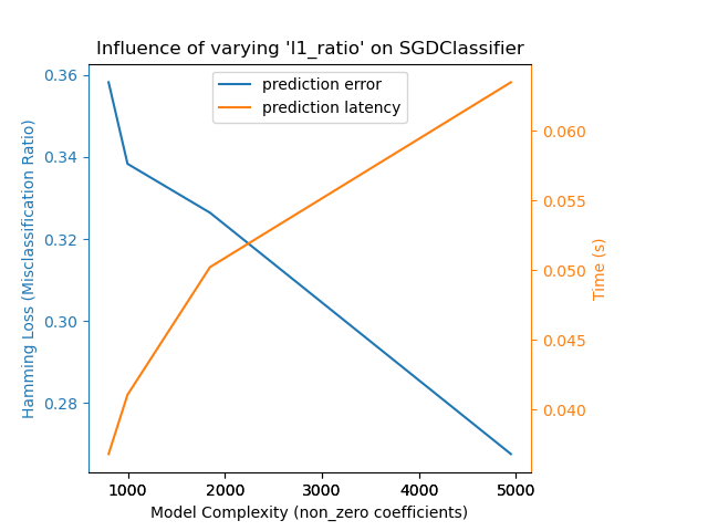
Benchmarking SGDClassifier(alpha=0.001, l1_ratio=0.25, loss='modified_huber',
              n_iter_no_change=2, penalty='elasticnet', tol=0.1)
Complexity: 4948 | Hamming Loss (Misclassification Ratio): 0.2675 | Pred. Time: 0.063463s

Benchmarking SGDClassifier(alpha=0.001, l1_ratio=0.5, loss='modified_huber',
              n_iter_no_change=2, penalty='elasticnet', tol=0.1)
Complexity: 1847 | Hamming Loss (Misclassification Ratio): 0.3264 | Pred. Time: 0.050223s

Benchmarking SGDClassifier(alpha=0.001, l1_ratio=0.75, loss='modified_huber',
              n_iter_no_change=2, penalty='elasticnet', tol=0.1)
Complexity: 997 | Hamming Loss (Misclassification Ratio): 0.3383 | Pred. Time: 0.041081s

Benchmarking SGDClassifier(alpha=0.001, l1_ratio=0.9, loss='modified_huber',
              n_iter_no_change=2, penalty='elasticnet', tol=0.1)
Complexity: 802 | Hamming Loss (Misclassification Ratio): 0.3582 | Pred. Time: 0.036837s

Benchmarking NuSVR(C=1000.0, gamma=3.0517578125e-05, nu=0.05)
Complexity: 18 | MSE: 5558.7313 | Pred. Time: 0.000400s

Benchmarking NuSVR(C=1000.0, gamma=3.0517578125e-05, nu=0.1)
Complexity: 36 | MSE: 5289.8022 | Pred. Time: 0.000312s

Benchmarking NuSVR(C=1000.0, gamma=3.0517578125e-05, nu=0.2)
Complexity: 72 | MSE: 5193.8353 | Pred. Time: 0.000466s

Benchmarking NuSVR(C=1000.0, gamma=3.0517578125e-05, nu=0.35)
Complexity: 124 | MSE: 5131.3279 | Pred. Time: 0.000672s

Benchmarking NuSVR(C=1000.0, gamma=3.0517578125e-05)
Complexity: 178 | MSE: 5149.0779 | Pred. Time: 0.000894s

Benchmarking GradientBoostingRegressor(learning_rate=0.05, max_depth=2, n_estimators=10)
Complexity: 10 | MSE: 4066.4812 | Pred. Time: 0.000459s

Benchmarking GradientBoostingRegressor(learning_rate=0.05, max_depth=2, n_estimators=25)
Complexity: 25 | MSE: 3551.1723 | Pred. Time: 0.000310s

Benchmarking GradientBoostingRegressor(learning_rate=0.05, max_depth=2, n_estimators=50)
Complexity: 50 | MSE: 3445.2171 | Pred. Time: 0.000352s

Benchmarking GradientBoostingRegressor(learning_rate=0.05, max_depth=2, n_estimators=75)
Complexity: 75 | MSE: 3433.0358 | Pred. Time: 0.000393s

Benchmarking GradientBoostingRegressor(learning_rate=0.05, max_depth=2)
Complexity: 100 | MSE: 3456.0602 | Pred. Time: 0.000426s
結論#
作為結論,我們可以推斷出以下見解
更複雜(或更具表現力)的模型將需要更長的訓練時間;
更複雜的模型並不保證能減少預測誤差。
這些方面與模型泛化以及避免模型欠擬合或過擬合有關。
腳本總執行時間: (0 分鐘 5.673 秒)
相關範例