使用 IterativeImputer 的變體填補遺失值#

IterativeImputer 類別非常靈活 - 它可以與各種估計器一起使用，以進行循環迴歸，將每個變數依次視為輸出。

在此範例中，我們比較了一些估計器，用於使用 IterativeImputer 進行遺失特徵填補

BayesianRidge：正規化線性迴歸
RandomForestRegressor：隨機樹迴歸森林
make_pipeline (Nystroem, Ridge)：具有 2 次多項式核心擴展和正規化線性迴歸的管道
KNeighborsRegressor：與其他 KNN 填補方法相當

特別令人感興趣的是 IterativeImputer 模仿 missForest 行為的能力，missForest 是 R 的熱門填補套件。

請注意，KNeighborsRegressor 與 KNN 填補不同，後者透過使用考慮遺失值的距離度量，從具有遺失值的樣本中學習，而不是填補它們。

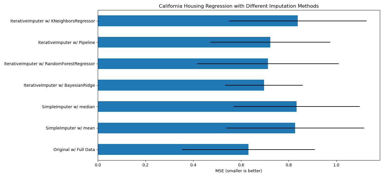
目標是比較不同的估計器，看看哪一個最適合 IterativeImputer，在每個列隨機刪除一個值的加州房屋資料集上使用 BayesianRidge 估計器時。

對於這種特定的遺失值模式，我們看到 BayesianRidge 和 RandomForestRegressor 給出最好的結果。

應該注意的是，一些估計器（例如 HistGradientBoostingRegressor）可以原生處理遺失特徵，並且通常建議使用它們，而不是建構具有複雜且成本高昂的遺失值填補策略的管道。

California Housing Regression with Different Imputation Methods

# Authors: The scikit-learn developers
# SPDX-License-Identifier: BSD-3-Clause

import matplotlib.pyplot as plt
import numpy as np
import pandas as pd

from sklearn.datasets import fetch_california_housing
from sklearn.ensemble import RandomForestRegressor

# To use this experimental feature, we need to explicitly ask for it:
from sklearn.experimental import enable_iterative_imputer  # noqa
from sklearn.impute import IterativeImputer, SimpleImputer
from sklearn.kernel_approximation import Nystroem
from sklearn.linear_model import BayesianRidge, Ridge
from sklearn.model_selection import cross_val_score
from sklearn.neighbors import KNeighborsRegressor
from sklearn.pipeline import make_pipeline

N_SPLITS = 5

rng = np.random.RandomState(0)

X_full, y_full = fetch_california_housing(return_X_y=True)
# ~2k samples is enough for the purpose of the example.
# Remove the following two lines for a slower run with different error bars.
X_full = X_full[::10]
y_full = y_full[::10]
n_samples, n_features = X_full.shape

# Estimate the score on the entire dataset, with no missing values
br_estimator = BayesianRidge()
score_full_data = pd.DataFrame(
    cross_val_score(
        br_estimator, X_full, y_full, scoring="neg_mean_squared_error", cv=N_SPLITS
    ),
    columns=["Full Data"],
)

# Add a single missing value to each row
X_missing = X_full.copy()
y_missing = y_full
missing_samples = np.arange(n_samples)
missing_features = rng.choice(n_features, n_samples, replace=True)
X_missing[missing_samples, missing_features] = np.nan

# Estimate the score after imputation (mean and median strategies)
score_simple_imputer = pd.DataFrame()
for strategy in ("mean", "median"):
    estimator = make_pipeline(
        SimpleImputer(missing_values=np.nan, strategy=strategy), br_estimator
    )
    score_simple_imputer[strategy] = cross_val_score(
        estimator, X_missing, y_missing, scoring="neg_mean_squared_error", cv=N_SPLITS
    )

# Estimate the score after iterative imputation of the missing values
# with different estimators
estimators = [
    BayesianRidge(),
    RandomForestRegressor(
        # We tuned the hyperparameters of the RandomForestRegressor to get a good
        # enough predictive performance for a restricted execution time.
        n_estimators=4,
        max_depth=10,
        bootstrap=True,
        max_samples=0.5,
        n_jobs=2,
        random_state=0,
    ),
    make_pipeline(
        Nystroem(kernel="polynomial", degree=2, random_state=0), Ridge(alpha=1e3)
    ),
    KNeighborsRegressor(n_neighbors=15),
]
score_iterative_imputer = pd.DataFrame()
# iterative imputer is sensible to the tolerance and
# dependent on the estimator used internally.
# we tuned the tolerance to keep this example run with limited computational
# resources while not changing the results too much compared to keeping the
# stricter default value for the tolerance parameter.
tolerances = (1e-3, 1e-1, 1e-1, 1e-2)
for impute_estimator, tol in zip(estimators, tolerances):
    estimator = make_pipeline(
        IterativeImputer(
            random_state=0, estimator=impute_estimator, max_iter=25, tol=tol
        ),
        br_estimator,
    )
    score_iterative_imputer[impute_estimator.__class__.__name__] = cross_val_score(
        estimator, X_missing, y_missing, scoring="neg_mean_squared_error", cv=N_SPLITS
    )

scores = pd.concat(
    [score_full_data, score_simple_imputer, score_iterative_imputer],
    keys=["Original", "SimpleImputer", "IterativeImputer"],
    axis=1,
)

# plot california housing results
fig, ax = plt.subplots(figsize=(13, 6))
means = -scores.mean()
errors = scores.std()
means.plot.barh(xerr=errors, ax=ax)
ax.set_title("California Housing Regression with Different Imputation Methods")
ax.set_xlabel("MSE (smaller is better)")
ax.set_yticks(np.arange(means.shape[0]))
ax.set_yticklabels([" w/ ".join(label) for label in means.index.tolist()])
plt.tight_layout(pad=1)
plt.show()