注意
前往結尾以下載完整的範例程式碼。或者透過 JupyterLite 或 Binder 在您的瀏覽器中執行此範例
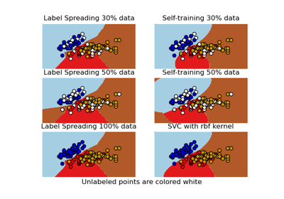
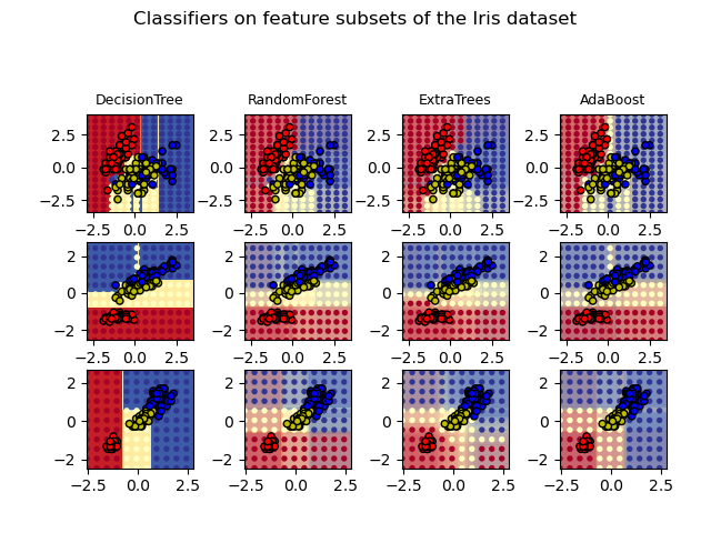
繪製樹集合在 Iris 資料集上的決策曲面#
繪製在 Iris 資料集特徵對上訓練的隨機樹森林的決策曲面。
此圖比較了決策樹分類器(第一欄)、隨機森林分類器(第二欄)、極端隨機樹分類器(第三欄)和 AdaBoost 分類器(第四欄)所學習的決策曲面。
在第一行中,分類器僅使用花萼寬度和花萼長度特徵建立,在第二行中僅使用花瓣長度和花萼長度,在第三行中僅使用花瓣寬度和花瓣長度。
當(在此範例之外)使用所有 4 個特徵、30 個估計器進行訓練,並使用 10 折交叉驗證進行評分時,依品質降序排列,我們看到
ExtraTreesClassifier()  # 0.95 score
RandomForestClassifier()  # 0.94 score
AdaBoost(DecisionTree(max_depth=3))  # 0.94 score
DecisionTree(max_depth=None)  # 0.94 score
增加 AdaBoost 的 max_depth 會降低分數的標準差(但平均分數不會提高)。
請參閱主控台的輸出,以取得每個模型的更多詳細資訊。
在此範例中,您可以嘗試
為
DecisionTreeClassifier和AdaBoostClassifier更改max_depth,也許為DecisionTreeClassifier嘗試max_depth=3或為AdaBoostClassifier嘗試max_depth=None變更
n_estimators
值得注意的是,RandomForests 和 ExtraTrees 可以並行在多個核心上進行擬合,因為每棵樹都是獨立於其他樹建立的。AdaBoost 的樣本是依序建立的,因此不使用多個核心。
DecisionTree with features [0, 1] has a score of 0.9266666666666666
RandomForest with 30 estimators with features [0, 1] has a score of 0.9266666666666666
ExtraTrees with 30 estimators with features [0, 1] has a score of 0.9266666666666666
AdaBoost with 30 estimators with features [0, 1] has a score of 0.82
DecisionTree with features [0, 2] has a score of 0.9933333333333333
RandomForest with 30 estimators with features [0, 2] has a score of 0.9933333333333333
ExtraTrees with 30 estimators with features [0, 2] has a score of 0.9933333333333333
AdaBoost with 30 estimators with features [0, 2] has a score of 0.9933333333333333
DecisionTree with features [2, 3] has a score of 0.9933333333333333
RandomForest with 30 estimators with features [2, 3] has a score of 0.9933333333333333
ExtraTrees with 30 estimators with features [2, 3] has a score of 0.9933333333333333
AdaBoost with 30 estimators with features [2, 3] has a score of 0.9866666666666667
# Authors: The scikit-learn developers
# SPDX-License-Identifier: BSD-3-Clause

import matplotlib.pyplot as plt
import numpy as np
from matplotlib.colors import ListedColormap

from sklearn.datasets import load_iris
from sklearn.ensemble import (
    AdaBoostClassifier,
    ExtraTreesClassifier,
    RandomForestClassifier,
)
from sklearn.tree import DecisionTreeClassifier

# Parameters
n_classes = 3
n_estimators = 30
cmap = plt.cm.RdYlBu
plot_step = 0.02  # fine step width for decision surface contours
plot_step_coarser = 0.5  # step widths for coarse classifier guesses
RANDOM_SEED = 13  # fix the seed on each iteration

# Load data
iris = load_iris()

plot_idx = 1

models = [
    DecisionTreeClassifier(max_depth=None),
    RandomForestClassifier(n_estimators=n_estimators),
    ExtraTreesClassifier(n_estimators=n_estimators),
    AdaBoostClassifier(DecisionTreeClassifier(max_depth=3), n_estimators=n_estimators),
]

for pair in ([0, 1], [0, 2], [2, 3]):
    for model in models:
        # We only take the two corresponding features
        X = iris.data[:, pair]
        y = iris.target

        # Shuffle
        idx = np.arange(X.shape[0])
        np.random.seed(RANDOM_SEED)
        np.random.shuffle(idx)
        X = X[idx]
        y = y[idx]

        # Standardize
        mean = X.mean(axis=0)
        std = X.std(axis=0)
        X = (X - mean) / std

        # Train
        model.fit(X, y)

        scores = model.score(X, y)
        # Create a title for each column and the console by using str() and
        # slicing away useless parts of the string
        model_title = str(type(model)).split(".")[-1][:-2][: -len("Classifier")]

        model_details = model_title
        if hasattr(model, "estimators_"):
            model_details += " with {} estimators".format(len(model.estimators_))
        print(model_details + " with features", pair, "has a score of", scores)

        plt.subplot(3, 4, plot_idx)
        if plot_idx <= len(models):
            # Add a title at the top of each column
            plt.title(model_title, fontsize=9)

        # Now plot the decision boundary using a fine mesh as input to a
        # filled contour plot
        x_min, x_max = X[:, 0].min() - 1, X[:, 0].max() + 1
        y_min, y_max = X[:, 1].min() - 1, X[:, 1].max() + 1
        xx, yy = np.meshgrid(
            np.arange(x_min, x_max, plot_step), np.arange(y_min, y_max, plot_step)
        )

        # Plot either a single DecisionTreeClassifier or alpha blend the
        # decision surfaces of the ensemble of classifiers
        if isinstance(model, DecisionTreeClassifier):
            Z = model.predict(np.c_[xx.ravel(), yy.ravel()])
            Z = Z.reshape(xx.shape)
            cs = plt.contourf(xx, yy, Z, cmap=cmap)
        else:
            # Choose alpha blend level with respect to the number
            # of estimators
            # that are in use (noting that AdaBoost can use fewer estimators
            # than its maximum if it achieves a good enough fit early on)
            estimator_alpha = 1.0 / len(model.estimators_)
            for tree in model.estimators_:
                Z = tree.predict(np.c_[xx.ravel(), yy.ravel()])
                Z = Z.reshape(xx.shape)
                cs = plt.contourf(xx, yy, Z, alpha=estimator_alpha, cmap=cmap)

        # Build a coarser grid to plot a set of ensemble classifications
        # to show how these are different to what we see in the decision
        # surfaces. These points are regularly space and do not have a
        # black outline
        xx_coarser, yy_coarser = np.meshgrid(
            np.arange(x_min, x_max, plot_step_coarser),
            np.arange(y_min, y_max, plot_step_coarser),
        )
        Z_points_coarser = model.predict(
            np.c_[xx_coarser.ravel(), yy_coarser.ravel()]
        ).reshape(xx_coarser.shape)
        cs_points = plt.scatter(
            xx_coarser,
            yy_coarser,
            s=15,
            c=Z_points_coarser,
            cmap=cmap,
            edgecolors="none",
        )

        # Plot the training points, these are clustered together and have a
        # black outline
        plt.scatter(
            X[:, 0],
            X[:, 1],
            c=y,
            cmap=ListedColormap(["r", "y", "b"]),
            edgecolor="k",
            s=20,
        )
        plot_idx += 1  # move on to the next plot in sequence

plt.suptitle("Classifiers on feature subsets of the Iris dataset", fontsize=12)
plt.axis("tight")
plt.tight_layout(h_pad=0.2, w_pad=0.2, pad=2.5)
plt.show()
腳本的總執行時間: (0 分鐘 7.719 秒)
相關範例