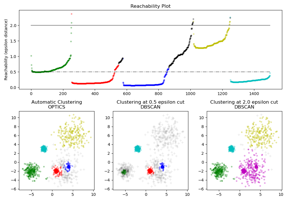
OPTICS 分群演算法的示範#

尋找高密度的核心樣本，並從這些樣本擴展集群。這個範例使用生成的資料，使群集具有不同的密度。

OPTICS 首先使用其 Xi 群集檢測方法，然後在可達性上設定特定閾值，這對應於 DBSCAN。我們可以觀察到，OPTICS 的 Xi 方法的不同群集可以透過 DBSCAN 中不同的閾值選擇來恢復。

Reachability Plot, Automatic Clustering OPTICS, Clustering at 0.5 epsilon cut DBSCAN, Clustering at 2.0 epsilon cut DBSCAN

# Authors: The scikit-learn developers
# SPDX-License-Identifier: BSD-3-Clause

import matplotlib.gridspec as gridspec
import matplotlib.pyplot as plt
import numpy as np

from sklearn.cluster import OPTICS, cluster_optics_dbscan

# Generate sample data

np.random.seed(0)
n_points_per_cluster = 250

C1 = [-5, -2] + 0.8 * np.random.randn(n_points_per_cluster, 2)
C2 = [4, -1] + 0.1 * np.random.randn(n_points_per_cluster, 2)
C3 = [1, -2] + 0.2 * np.random.randn(n_points_per_cluster, 2)
C4 = [-2, 3] + 0.3 * np.random.randn(n_points_per_cluster, 2)
C5 = [3, -2] + 1.6 * np.random.randn(n_points_per_cluster, 2)
C6 = [5, 6] + 2 * np.random.randn(n_points_per_cluster, 2)
X = np.vstack((C1, C2, C3, C4, C5, C6))

clust = OPTICS(min_samples=50, xi=0.05, min_cluster_size=0.05)

# Run the fit
clust.fit(X)

labels_050 = cluster_optics_dbscan(
    reachability=clust.reachability_,
    core_distances=clust.core_distances_,
    ordering=clust.ordering_,
    eps=0.5,
)
labels_200 = cluster_optics_dbscan(
    reachability=clust.reachability_,
    core_distances=clust.core_distances_,
    ordering=clust.ordering_,
    eps=2,
)

space = np.arange(len(X))
reachability = clust.reachability_[clust.ordering_]
labels = clust.labels_[clust.ordering_]

plt.figure(figsize=(10, 7))
G = gridspec.GridSpec(2, 3)
ax1 = plt.subplot(G[0, :])
ax2 = plt.subplot(G[1, 0])
ax3 = plt.subplot(G[1, 1])
ax4 = plt.subplot(G[1, 2])

# Reachability plot
colors = ["g.", "r.", "b.", "y.", "c."]
for klass, color in enumerate(colors):
    Xk = space[labels == klass]
    Rk = reachability[labels == klass]
    ax1.plot(Xk, Rk, color, alpha=0.3)
ax1.plot(space[labels == -1], reachability[labels == -1], "k.", alpha=0.3)
ax1.plot(space, np.full_like(space, 2.0, dtype=float), "k-", alpha=0.5)
ax1.plot(space, np.full_like(space, 0.5, dtype=float), "k-.", alpha=0.5)
ax1.set_ylabel("Reachability (epsilon distance)")
ax1.set_title("Reachability Plot")

# OPTICS
colors = ["g.", "r.", "b.", "y.", "c."]
for klass, color in enumerate(colors):
    Xk = X[clust.labels_ == klass]
    ax2.plot(Xk[:, 0], Xk[:, 1], color, alpha=0.3)
ax2.plot(X[clust.labels_ == -1, 0], X[clust.labels_ == -1, 1], "k+", alpha=0.1)
ax2.set_title("Automatic Clustering\nOPTICS")

# DBSCAN at 0.5
colors = ["g.", "r.", "b.", "c."]
for klass, color in enumerate(colors):
    Xk = X[labels_050 == klass]
    ax3.plot(Xk[:, 0], Xk[:, 1], color, alpha=0.3)
ax3.plot(X[labels_050 == -1, 0], X[labels_050 == -1, 1], "k+", alpha=0.1)
ax3.set_title("Clustering at 0.5 epsilon cut\nDBSCAN")

# DBSCAN at 2.
colors = ["g.", "m.", "y.", "c."]
for klass, color in enumerate(colors):
    Xk = X[labels_200 == klass]
    ax4.plot(Xk[:, 0], Xk[:, 1], color, alpha=0.3)
ax4.plot(X[labels_200 == -1, 0], X[labels_200 == -1, 1], "k+", alpha=0.1)
ax4.set_title("Clustering at 2.0 epsilon cut\nDBSCAN")

plt.tight_layout()
plt.show()