注意
跳到結尾 以下載完整的範例程式碼。或透過 JupyterLite 或 Binder 在您的瀏覽器中執行此範例
等張迴歸#
在生成的數據上(具有同方差均勻雜訊的非線性單調趨勢)等張迴歸的說明。
等張迴歸演算法找到一個函數的非遞減近似值,同時最小化訓練數據上的均方誤差。這種非參數模型的好處是它不假設目標函數有任何形狀,除了單調性。為比較起見,也提出了線性迴歸。
右側的圖顯示了模型預測函數,該函數是由閾值點的線性插值產生的。閾值點是訓練輸入觀察的子集,它們的匹配目標值由等張非參數擬合計算得出。
# Authors: The scikit-learn developers
# SPDX-License-Identifier: BSD-3-Clause

import matplotlib.pyplot as plt
import numpy as np
from matplotlib.collections import LineCollection

from sklearn.isotonic import IsotonicRegression
from sklearn.linear_model import LinearRegression
from sklearn.utils import check_random_state

n = 100
x = np.arange(n)
rs = check_random_state(0)
y = rs.randint(-50, 50, size=(n,)) + 50.0 * np.log1p(np.arange(n))
擬合 IsotonicRegression 和 LinearRegression 模型
ir = IsotonicRegression(out_of_bounds="clip")
y_ = ir.fit_transform(x, y)

lr = LinearRegression()
lr.fit(x[:, np.newaxis], y)  # x needs to be 2d for LinearRegression
繪製結果
segments = [[[i, y[i]], [i, y_[i]]] for i in range(n)]
lc = LineCollection(segments, zorder=0)
lc.set_array(np.ones(len(y)))
lc.set_linewidths(np.full(n, 0.5))

fig, (ax0, ax1) = plt.subplots(ncols=2, figsize=(12, 6))

ax0.plot(x, y, "C0.", markersize=12)
ax0.plot(x, y_, "C1.-", markersize=12)
ax0.plot(x, lr.predict(x[:, np.newaxis]), "C2-")
ax0.add_collection(lc)
ax0.legend(("Training data", "Isotonic fit", "Linear fit"), loc="lower right")
ax0.set_title("Isotonic regression fit on noisy data (n=%d)" % n)

x_test = np.linspace(-10, 110, 1000)
ax1.plot(x_test, ir.predict(x_test), "C1-")
ax1.plot(ir.X_thresholds_, ir.y_thresholds_, "C1.", markersize=12)
ax1.set_title("Prediction function (%d thresholds)" % len(ir.X_thresholds_))

plt.show()
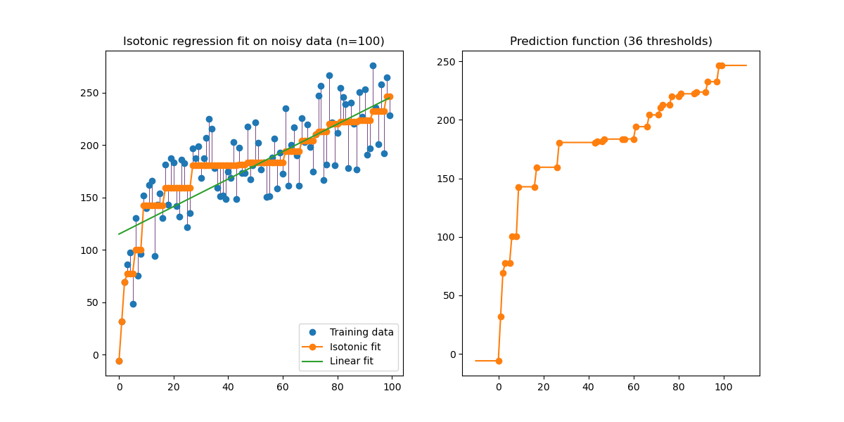
請注意,我們明確地將 out_of_bounds="clip" 傳遞給 IsotonicRegression 的建構函式,以控制模型在訓練集中觀察到的數據範圍之外的外推方式。這種「剪輯」外推可以在右側的決策函數圖上看到。
腳本的總執行時間:(0 分鐘 0.150 秒)
相關範例