注意
前往結尾下載完整範例程式碼。 或透過 JupyterLite 或 Binder 在您的瀏覽器中執行此範例
多項式和一對多邏輯迴歸的決策邊界#
此範例比較了多項式和一對多邏輯迴歸在具有三個類別的 2D 數據集上的決策邊界。
我們對兩種方法的決策邊界進行比較,這相當於呼叫方法 predict。 此外,我們繪製了對應於類別機率估計為 0.5 時的線的超平面。
# Authors: The scikit-learn developers
# SPDX-License-Identifier: BSD-3-Clause
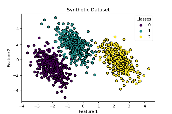
數據集生成#
我們使用 make_blobs 函數生成合成數據集。 數據集由來自三個不同類別的 1,000 個樣本組成,中心分別在 [-5, 0]、[0, 1.5] 和 [5, -1] 附近。 生成後,我們應用線性變換以引入特徵之間的一些相關性,並使問題更具挑戰性。 這會產生一個具有三個重疊類別的 2D 數據集,適用於展示多項式和一對多邏輯迴歸之間的差異。
import matplotlib.pyplot as plt
import numpy as np

from sklearn.datasets import make_blobs

centers = [[-5, 0], [0, 1.5], [5, -1]]
X, y = make_blobs(n_samples=1_000, centers=centers, random_state=40)
transformation = [[0.4, 0.2], [-0.4, 1.2]]
X = np.dot(X, transformation)

fig, ax = plt.subplots(figsize=(6, 4))

scatter = ax.scatter(X[:, 0], X[:, 1], c=y, edgecolor="black")
ax.set(title="Synthetic Dataset", xlabel="Feature 1", ylabel="Feature 2")
_ = ax.legend(*scatter.legend_elements(), title="Classes")
分類器訓練#
我們訓練兩個不同的邏輯迴歸分類器:多項式和一對多。 多項式分類器同時處理所有類別,而一對多方法則針對每個類別訓練一個二元分類器,以對抗所有其他類別。
from sklearn.linear_model import LogisticRegression
from sklearn.multiclass import OneVsRestClassifier

logistic_regression_multinomial = LogisticRegression().fit(X, y)
logistic_regression_ovr = OneVsRestClassifier(LogisticRegression()).fit(X, y)

accuracy_multinomial = logistic_regression_multinomial.score(X, y)
accuracy_ovr = logistic_regression_ovr.score(X, y)
決策邊界視覺化#
讓我們視覺化由分類器的 predict 方法提供的兩個模型的決策邊界。
from sklearn.inspection import DecisionBoundaryDisplay

fig, (ax1, ax2) = plt.subplots(1, 2, figsize=(12, 5), sharex=True, sharey=True)

for model, title, ax in [
    (
        logistic_regression_multinomial,
        f"Multinomial Logistic Regression\n(Accuracy: {accuracy_multinomial:.3f})",
        ax1,
    ),
    (
        logistic_regression_ovr,
        f"One-vs-Rest Logistic Regression\n(Accuracy: {accuracy_ovr:.3f})",
        ax2,
    ),
]:
    DecisionBoundaryDisplay.from_estimator(
        model,
        X,
        ax=ax,
        response_method="predict",
        alpha=0.8,
    )
    scatter = ax.scatter(X[:, 0], X[:, 1], c=y, edgecolor="k")
    legend = ax.legend(*scatter.legend_elements(), title="Classes")
    ax.add_artist(legend)
    ax.set_title(title)
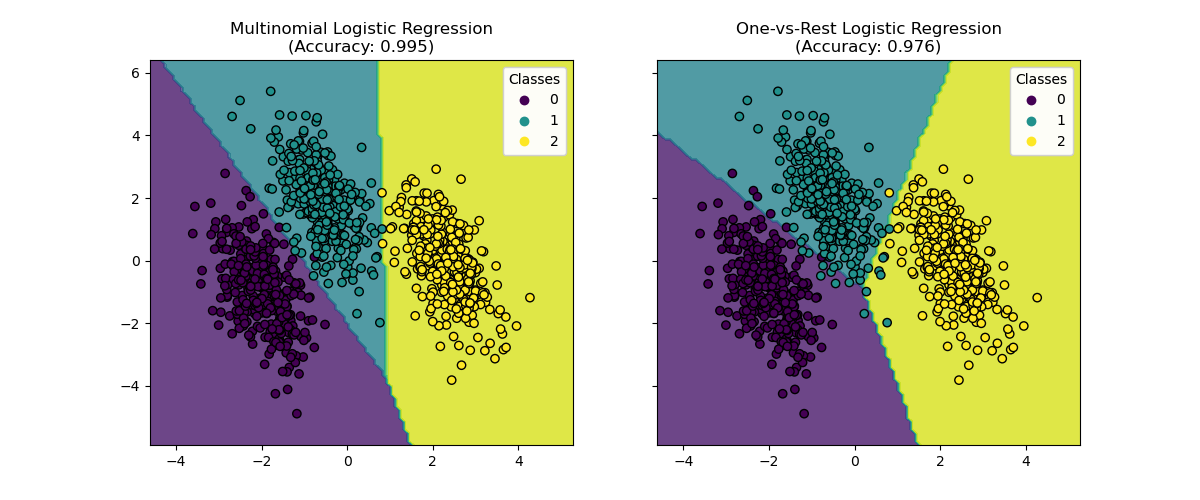
我們看到決策邊界是不同的。 這種差異源於它們的方法
多項式邏輯迴歸在優化期間同時考慮所有類別。
一對多邏輯迴歸針對每個類別獨立擬合以對抗所有其他類別。
這些不同的策略可能會導致不同的決策邊界,尤其是在複雜的多類別問題中。
超平面視覺化#
我們還視覺化了當類別機率估計為 0.5 時對應於線的超平面。
def plot_hyperplanes(classifier, X, ax):
    xmin, xmax = X[:, 0].min(), X[:, 0].max()
    ymin, ymax = X[:, 1].min(), X[:, 1].max()
    ax.set(xlim=(xmin, xmax), ylim=(ymin, ymax))

    if isinstance(classifier, OneVsRestClassifier):
        coef = np.concatenate([est.coef_ for est in classifier.estimators_])
        intercept = np.concatenate([est.intercept_ for est in classifier.estimators_])
    else:
        coef = classifier.coef_
        intercept = classifier.intercept_

    for i in range(coef.shape[0]):
        w = coef[i]
        a = -w[0] / w[1]
        xx = np.linspace(xmin, xmax)
        yy = a * xx - (intercept[i]) / w[1]
        ax.plot(xx, yy, "--", linewidth=3, label=f"Class {i}")

    return ax.get_legend_handles_labels()
fig, (ax1, ax2) = plt.subplots(1, 2, figsize=(12, 5), sharex=True, sharey=True)

for model, title, ax in [
    (
        logistic_regression_multinomial,
        "Multinomial Logistic Regression Hyperplanes",
        ax1,
    ),
    (logistic_regression_ovr, "One-vs-Rest Logistic Regression Hyperplanes", ax2),
]:
    hyperplane_handles, hyperplane_labels = plot_hyperplanes(model, X, ax)
    scatter = ax.scatter(X[:, 0], X[:, 1], c=y, edgecolor="k")
    scatter_handles, scatter_labels = scatter.legend_elements()

    all_handles = hyperplane_handles + scatter_handles
    all_labels = hyperplane_labels + scatter_labels

    ax.legend(all_handles, all_labels, title="Classes")
    ax.set_title(title)

plt.show()
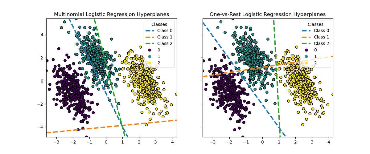
雖然兩種方法之間類別 0 和 2 的超平面非常相似,但我們觀察到類別 1 的超平面明顯不同。 這種差異源於一對多和多項式邏輯迴歸的基本方法
對於一對多邏輯迴歸
每個超平面都是通過考慮一個類別與所有其他類別來獨立確定的。
對於類別 1,超平面表示最佳將類別 1 與類別 0 和 2 的組合分開的決策邊界。
這種二元方法可能會導致更簡單的決策邊界,但可能無法同時捕獲所有類別之間的複雜關係。
無法解釋條件類別機率。
對於多項式邏輯迴歸
所有超平面都是同時確定的,同時考慮所有類別之間的關係。
模型最小化的損失是一個適當的評分規則,這表示模型已針對估計有意義的條件類別機率進行最佳化。
每個超平面表示一個決策邊界,其中一個類別的機率基於整體機率分佈高於其他類別。
這種方法可以捕獲類別之間更細微的關係,可能會在多類別問題中產生更準確的分類。
超平面的差異,尤其是類別 1 的差異,突顯了這些方法如何在整體準確性相似的情況下產生不同的決策邊界。
在實踐中,建議使用多項式邏輯迴歸,因為它最小化了明確定義的損失函數,從而產生了更好的校準類別機率,並因此產生了更易於解釋的結果。 在決策邊界方面,應制定一個效用函數,將類別機率轉換為手頭問題的有意義的量。 一對多允許不同的決策邊界,但不允許像效用函數那樣對類別之間的權衡進行精細控制。
腳本的總運行時間: (0 分鐘 0.628 秒)
相關範例