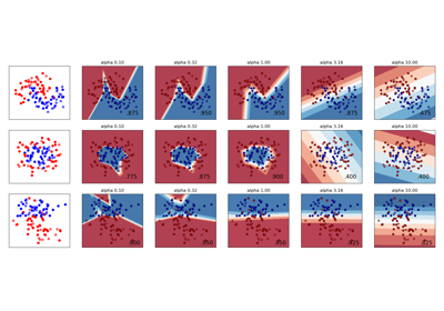
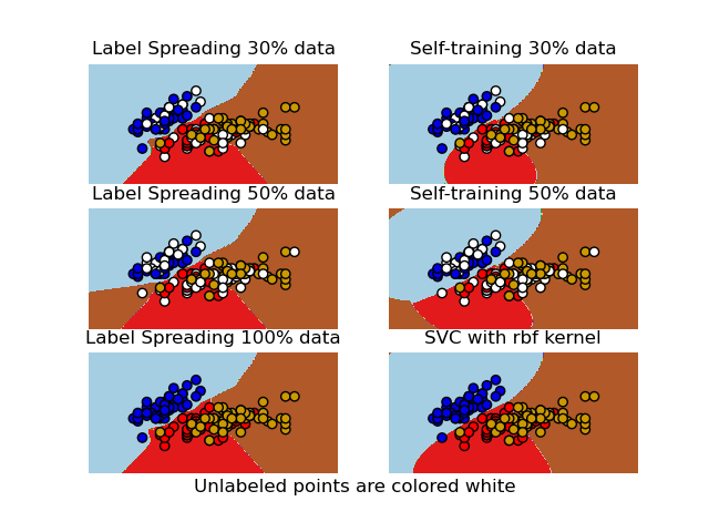
半監督分類器與 SVM 在 Iris 資料集上的決策邊界#

比較標籤傳播、自訓練和 SVM 在 iris 資料集上產生的決策邊界。

此範例示範即使在少量標記資料可用的情況下，標籤傳播和自訓練也可以學習良好的邊界。

請注意，省略了使用 100% 資料的自訓練，因為它在功能上與在 100% 資料上訓練 SVC 相同。

Unlabeled points are colored white, Label Spreading 30% data, Self-training 30% data, Label Spreading 50% data, Self-training 50% data, Label Spreading 100% data, SVC with rbf kernel

# Authors: The scikit-learn developers
# SPDX-License-Identifier: BSD-3-Clause

import matplotlib.pyplot as plt
import numpy as np

from sklearn import datasets
from sklearn.semi_supervised import LabelSpreading, SelfTrainingClassifier
from sklearn.svm import SVC

iris = datasets.load_iris()

X = iris.data[:, :2]
y = iris.target

# step size in the mesh
h = 0.02

rng = np.random.RandomState(0)
y_rand = rng.rand(y.shape[0])
y_30 = np.copy(y)
y_30[y_rand < 0.3] = -1  # set random samples to be unlabeled
y_50 = np.copy(y)
y_50[y_rand < 0.5] = -1
# we create an instance of SVM and fit out data. We do not scale our
# data since we want to plot the support vectors
ls30 = (LabelSpreading().fit(X, y_30), y_30, "Label Spreading 30% data")
ls50 = (LabelSpreading().fit(X, y_50), y_50, "Label Spreading 50% data")
ls100 = (LabelSpreading().fit(X, y), y, "Label Spreading 100% data")

# the base classifier for self-training is identical to the SVC
base_classifier = SVC(kernel="rbf", gamma=0.5, probability=True)
st30 = (
    SelfTrainingClassifier(base_classifier).fit(X, y_30),
    y_30,
    "Self-training 30% data",
)
st50 = (
    SelfTrainingClassifier(base_classifier).fit(X, y_50),
    y_50,
    "Self-training 50% data",
)

rbf_svc = (SVC(kernel="rbf", gamma=0.5).fit(X, y), y, "SVC with rbf kernel")

# create a mesh to plot in
x_min, x_max = X[:, 0].min() - 1, X[:, 0].max() + 1
y_min, y_max = X[:, 1].min() - 1, X[:, 1].max() + 1
xx, yy = np.meshgrid(np.arange(x_min, x_max, h), np.arange(y_min, y_max, h))

color_map = {-1: (1, 1, 1), 0: (0, 0, 0.9), 1: (1, 0, 0), 2: (0.8, 0.6, 0)}

classifiers = (ls30, st30, ls50, st50, ls100, rbf_svc)
for i, (clf, y_train, title) in enumerate(classifiers):
    # Plot the decision boundary. For that, we will assign a color to each
    # point in the mesh [x_min, x_max]x[y_min, y_max].
    plt.subplot(3, 2, i + 1)
    Z = clf.predict(np.c_[xx.ravel(), yy.ravel()])

    # Put the result into a color plot
    Z = Z.reshape(xx.shape)
    plt.contourf(xx, yy, Z, cmap=plt.cm.Paired)
    plt.axis("off")

    # Plot also the training points
    colors = [color_map[y] for y in y_train]
    plt.scatter(X[:, 0], X[:, 1], c=colors, edgecolors="black")

    plt.title(title)

plt.suptitle("Unlabeled points are colored white", y=0.1)
plt.show()