穩健共變異數估計和馬氏距離的相關性#

此範例顯示高斯分佈資料的馬氏距離的共變異數估計。

對於高斯分佈資料，可以使用馬氏距離計算觀測值 \(x_i\) 到分佈模式的距離

\[d_{(\mu,\Sigma)}(x_i)^2 = (x_i - \mu)^T\Sigma^{-1}(x_i - \mu)\]

其中 \(\mu\) 和 \(\Sigma\) 是基礎高斯分佈的位置和共變異數。

實際上，\(\mu\) 和 \(\Sigma\) 由某些估計值取代。標準共變異數最大概似估計 (MLE) 對資料集中離群值的存在非常敏感，因此，下游馬氏距離也是如此。最好使用穩健的共變異數估計器，以確保估計值能夠抵抗資料集中的「錯誤」觀測值，並且計算出的馬氏距離能夠準確反映觀測值的真實組織。

最小共變異數行列式估計器 (MCD) 是一種穩健的高崩潰點（即它可用於估計高污染資料集的共變異數矩陣，最多可達 \(\frac{n_\text{samples}-n_\text{features}-1}{2}\) 個離群值）共變異數估計器。MCD 背後的概念是找到 \(\frac{n_\text{samples}+n_\text{features}+1}{2}\) 個觀測值，這些觀測值的經驗共變異數具有最小行列式，從而產生「純」觀測值子集，從中計算位置和共變異數的標準估計值。MCD 由 P.J.Rousseuw 在 [1] 中提出。

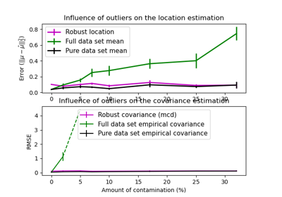
此範例說明馬氏距離如何受到離群資料的影響。當使用基於標準共變異數 MLE 的馬氏距離時，從污染分佈中繪製的觀測值與來自真實高斯分佈的觀測值無法區分。使用基於 MCD 的馬氏距離，兩個群體變得可以區分。相關應用包括離群值檢測、觀測值排名和分群。

注意

另請參閱穩健與經驗共變異數估計

參考文獻

# Authors: The scikit-learn developers
# SPDX-License-Identifier: BSD-3-Clause

產生資料#

首先，我們產生一個包含 125 個樣本和 2 個特徵的資料集。兩個特徵都是高斯分佈，平均值為 0，但特徵 1 的標準差等於 2，而特徵 2 的標準差等於 1。接下來，25 個樣本被高斯離群值樣本取代，其中特徵 1 的標準差等於 1，而特徵 2 的標準差等於 7。

import numpy as np

# for consistent results
np.random.seed(7)

n_samples = 125
n_outliers = 25
n_features = 2

# generate Gaussian data of shape (125, 2)
gen_cov = np.eye(n_features)
gen_cov[0, 0] = 2.0
X = np.dot(np.random.randn(n_samples, n_features), gen_cov)
# add some outliers
outliers_cov = np.eye(n_features)
outliers_cov[np.arange(1, n_features), np.arange(1, n_features)] = 7.0
X[-n_outliers:] = np.dot(np.random.randn(n_outliers, n_features), outliers_cov)

結果比較#

在下面，我們將基於 MCD 和 MLE 的共變異數估計器擬合到我們的資料，並列印估計的共變異數矩陣。請注意，基於 MLE 的估計器（7.5）的特徵 2 的估計變異數比 MCD 穩健估計器（1.2）的估計變異數高得多。這表明，基於 MCD 的穩健估計器更能抵抗離群值樣本，這些樣本的特徵 2 具有更大的變異數。

import matplotlib.pyplot as plt

from sklearn.covariance import EmpiricalCovariance, MinCovDet

# fit a MCD robust estimator to data
robust_cov = MinCovDet().fit(X)
# fit a MLE estimator to data
emp_cov = EmpiricalCovariance().fit(X)
print(
    "Estimated covariance matrix:\nMCD (Robust):\n{}\nMLE:\n{}".format(
        robust_cov.covariance_, emp_cov.covariance_
    )
)

Estimated covariance matrix:
MCD (Robust):
[[ 3.26253567e+00 -3.06695631e-03]
 [-3.06695631e-03  1.22747343e+00]]
MLE:
[[ 3.23773583 -0.24640578]
 [-0.24640578  7.51963999]]

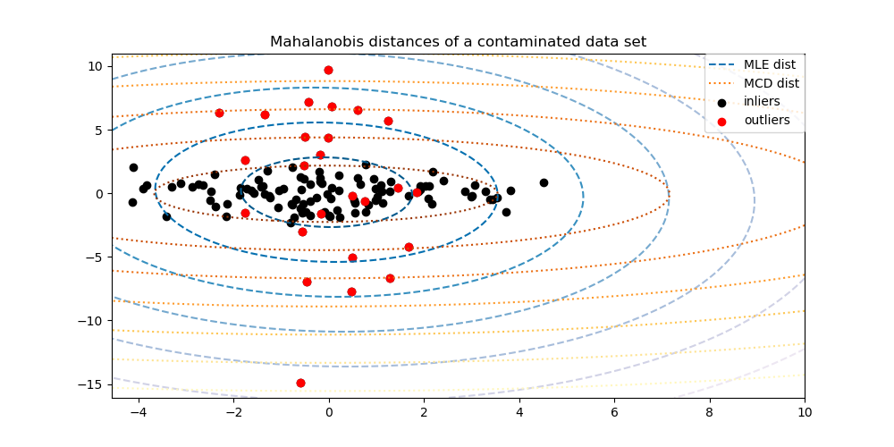
為了更好地視覺化差異，我們繪製由兩種方法計算出的馬氏距離的等高線。請注意，基於穩健 MCD 的馬氏距離更適合內點黑點，而基於 MLE 的距離則更容易受到離群值紅點的影響。

import matplotlib.lines as mlines

fig, ax = plt.subplots(figsize=(10, 5))
# Plot data set
inlier_plot = ax.scatter(X[:, 0], X[:, 1], color="black", label="inliers")
outlier_plot = ax.scatter(
    X[:, 0][-n_outliers:], X[:, 1][-n_outliers:], color="red", label="outliers"
)
ax.set_xlim(ax.get_xlim()[0], 10.0)
ax.set_title("Mahalanobis distances of a contaminated data set")

# Create meshgrid of feature 1 and feature 2 values
xx, yy = np.meshgrid(
    np.linspace(plt.xlim()[0], plt.xlim()[1], 100),
    np.linspace(plt.ylim()[0], plt.ylim()[1], 100),
)
zz = np.c_[xx.ravel(), yy.ravel()]
# Calculate the MLE based Mahalanobis distances of the meshgrid
mahal_emp_cov = emp_cov.mahalanobis(zz)
mahal_emp_cov = mahal_emp_cov.reshape(xx.shape)
emp_cov_contour = plt.contour(
    xx, yy, np.sqrt(mahal_emp_cov), cmap=plt.cm.PuBu_r, linestyles="dashed"
)
# Calculate the MCD based Mahalanobis distances
mahal_robust_cov = robust_cov.mahalanobis(zz)
mahal_robust_cov = mahal_robust_cov.reshape(xx.shape)
robust_contour = ax.contour(
    xx, yy, np.sqrt(mahal_robust_cov), cmap=plt.cm.YlOrBr_r, linestyles="dotted"
)

# Add legend
ax.legend(
    [
        mlines.Line2D([], [], color="tab:blue", linestyle="dashed"),
        mlines.Line2D([], [], color="tab:orange", linestyle="dotted"),
        inlier_plot,
        outlier_plot,
    ],
    ["MLE dist", "MCD dist", "inliers", "outliers"],
    loc="upper right",
    borderaxespad=0,
)

plt.show()

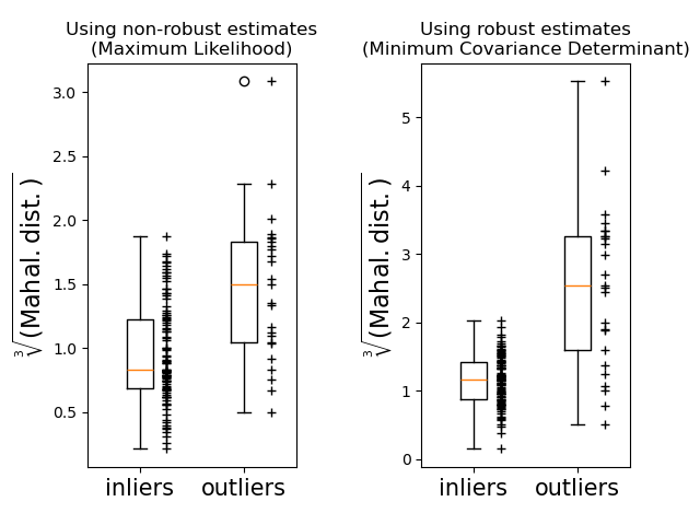
Mahalanobis distances of a contaminated data set

最後，我們強調基於 MCD 的馬氏距離區分離群值的能力。我們取馬氏距離的立方根，產生近似常態分佈（如 Wilson 和 Hilferty [2] 所建議），然後使用盒狀圖繪製內點和離群值樣本的值。對於基於穩健 MCD 的馬氏距離，離群值樣本的分佈與內點樣本的分佈更為分離。

fig, (ax1, ax2) = plt.subplots(1, 2)
plt.subplots_adjust(wspace=0.6)

# Calculate cubic root of MLE Mahalanobis distances for samples
emp_mahal = emp_cov.mahalanobis(X - np.mean(X, 0)) ** (0.33)
# Plot boxplots
ax1.boxplot([emp_mahal[:-n_outliers], emp_mahal[-n_outliers:]], widths=0.25)
# Plot individual samples
ax1.plot(
    np.full(n_samples - n_outliers, 1.26),
    emp_mahal[:-n_outliers],
    "+k",
    markeredgewidth=1,
)
ax1.plot(np.full(n_outliers, 2.26), emp_mahal[-n_outliers:], "+k", markeredgewidth=1)
ax1.axes.set_xticklabels(("inliers", "outliers"), size=15)
ax1.set_ylabel(r"$\sqrt[3]{\rm{(Mahal. dist.)}}$", size=16)
ax1.set_title("Using non-robust estimates\n(Maximum Likelihood)")

# Calculate cubic root of MCD Mahalanobis distances for samples
robust_mahal = robust_cov.mahalanobis(X - robust_cov.location_) ** (0.33)
# Plot boxplots
ax2.boxplot([robust_mahal[:-n_outliers], robust_mahal[-n_outliers:]], widths=0.25)
# Plot individual samples
ax2.plot(
    np.full(n_samples - n_outliers, 1.26),
    robust_mahal[:-n_outliers],
    "+k",
    markeredgewidth=1,
)
ax2.plot(np.full(n_outliers, 2.26), robust_mahal[-n_outliers:], "+k", markeredgewidth=1)
ax2.axes.set_xticklabels(("inliers", "outliers"), size=15)
ax2.set_ylabel(r"$\sqrt[3]{\rm{(Mahal. dist.)}}$", size=16)
ax2.set_title("Using robust estimates\n(Minimum Covariance Determinant)")

plt.show()