使用交叉驗證的遞迴特徵消除#

一個遞迴特徵消除 (RFE) 範例，具有使用交叉驗證自動調整選取特徵的數量。

# Authors: The scikit-learn developers
# SPDX-License-Identifier: BSD-3-Clause

資料產生#

我們使用 3 個資訊豐富的特徵建立分類任務。引入 2 個額外的冗餘（即相關）特徵的效果是，選取的特徵會根據交叉驗證的摺疊而變化。其餘的特徵不具資訊性，因為它們是隨機繪製的。

from sklearn.datasets import make_classification

X, y = make_classification(
    n_samples=500,
    n_features=15,
    n_informative=3,
    n_redundant=2,
    n_repeated=0,
    n_classes=8,
    n_clusters_per_class=1,
    class_sep=0.8,
    random_state=0,
)

模型訓練和選取#

我們建立 RFE 物件並計算交叉驗證分數。評分策略「準確率」可最佳化正確分類樣本的比例。

from sklearn.feature_selection import RFECV
from sklearn.linear_model import LogisticRegression
from sklearn.model_selection import StratifiedKFold

min_features_to_select = 1  # Minimum number of features to consider
clf = LogisticRegression()
cv = StratifiedKFold(5)

rfecv = RFECV(
    estimator=clf,
    step=1,
    cv=cv,
    scoring="accuracy",
    min_features_to_select=min_features_to_select,
    n_jobs=2,
)
rfecv.fit(X, y)

print(f"Optimal number of features: {rfecv.n_features_}")

Optimal number of features: 3

在本例中，發現具有 3 個特徵（對應於真正的生成模型）的模型是最理想的。

繪製特徵數量與交叉驗證分數的關係圖#

import matplotlib.pyplot as plt
import pandas as pd

cv_results = pd.DataFrame(rfecv.cv_results_)
plt.figure()
plt.xlabel("Number of features selected")
plt.ylabel("Mean test accuracy")
plt.errorbar(
    x=cv_results["n_features"],
    y=cv_results["mean_test_score"],
    yerr=cv_results["std_test_score"],
)
plt.title("Recursive Feature Elimination \nwith correlated features")
plt.show()

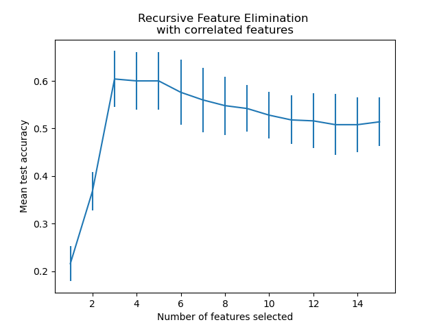
Recursive Feature Elimination with correlated features

從上面的圖中，可以進一步注意到，對於 3 到 5 個選取的特徵，等效分數會出現高原期（相似的平均值和重疊的誤差線）。這是引入相關特徵的結果。實際上，RFE 選取的最佳模型可能位於此範圍內，具體取決於交叉驗證技術。測試準確性在選取 5 個以上特徵時會降低，也就是說，保留不具資訊性的特徵會導致過度擬合，因此不利於模型的統計效能。

腳本的總執行時間：(0 分鐘 0.523 秒)