注意
前往末尾以下載完整範例程式碼,或透過 JupyterLite 或 Binder 在您的瀏覽器中執行此範例
梯度提升中的提前停止#
梯度提升是一種集成技術,它結合多個弱學習器(通常是決策樹)來創建穩健且強大的預測模型。它是以迭代方式進行的,其中每個新的階段(樹)都會修正前一個階段的錯誤。
提前停止是梯度提升中的一種技術,可讓我們找到建立一個能很好地推廣到未見資料並避免過擬合的模型所需的最佳迭代次數。這個概念很簡單:我們將資料集的一部分保留為驗證集(使用 validation_fraction 指定),以評估模型在訓練期間的效能。當模型透過額外的階段(樹)迭代建置時,會監控其在驗證集上的效能,作為步驟數的函數。
當模型在驗證集上的效能連續多個階段(由 n_iter_no_change 指定)內達到平穩狀態或惡化時(在 tol 指定的偏差範圍內),提前停止會生效。這表示模型已達到一個點,其中進一步的迭代可能會導致過擬合,並且是時候停止訓練了。
當應用提前停止時,最終模型中估計器(樹)的數量可以使用 n_estimators_ 屬性存取。總體而言,提前停止是在梯度提升中在模型效能和效率之間取得平衡的寶貴工具。
授權:BSD 3 條款
# Authors: The scikit-learn developers
# SPDX-License-Identifier: BSD-3-Clause
資料準備#
首先,我們載入並準備加州房價資料集以進行訓練和評估。它會對資料集進行子集化,並將其拆分為訓練集和驗證集。
import time

import matplotlib.pyplot as plt

from sklearn.datasets import fetch_california_housing
from sklearn.ensemble import GradientBoostingRegressor
from sklearn.metrics import mean_squared_error
from sklearn.model_selection import train_test_split

data = fetch_california_housing()
X, y = data.data[:600], data.target[:600]

X_train, X_val, y_train, y_val = train_test_split(X, y, test_size=0.2, random_state=42)
模型訓練與比較#
訓練兩個 GradientBoostingRegressor 模型:一個使用提前停止,另一個不使用。目的是比較它們的效能。它也會計算訓練時間和兩個模型使用的 n_estimators_。
params = dict(n_estimators=1000, max_depth=5, learning_rate=0.1, random_state=42)

gbm_full = GradientBoostingRegressor(**params)
gbm_early_stopping = GradientBoostingRegressor(
    **params,
    validation_fraction=0.1,
    n_iter_no_change=10,
)

start_time = time.time()
gbm_full.fit(X_train, y_train)
training_time_full = time.time() - start_time
n_estimators_full = gbm_full.n_estimators_

start_time = time.time()
gbm_early_stopping.fit(X_train, y_train)
training_time_early_stopping = time.time() - start_time
estimators_early_stopping = gbm_early_stopping.n_estimators_
錯誤計算#
此程式碼會計算先前章節中訓練的模型在訓練和驗證資料集上的 mean_squared_error。它會計算每個提升迭代的錯誤。目的是評估模型的效能和收斂性。
train_errors_without = []
val_errors_without = []

train_errors_with = []
val_errors_with = []

for i, (train_pred, val_pred) in enumerate(
    zip(
        gbm_full.staged_predict(X_train),
        gbm_full.staged_predict(X_val),
    )
):
    train_errors_without.append(mean_squared_error(y_train, train_pred))
    val_errors_without.append(mean_squared_error(y_val, val_pred))

for i, (train_pred, val_pred) in enumerate(
    zip(
        gbm_early_stopping.staged_predict(X_train),
        gbm_early_stopping.staged_predict(X_val),
    )
):
    train_errors_with.append(mean_squared_error(y_train, train_pred))
    val_errors_with.append(mean_squared_error(y_val, val_pred))
視覺化比較#
它包括三個子圖
繪製兩個模型在提升迭代中的訓練錯誤。
繪製兩個模型在提升迭代中的驗證錯誤。
建立長條圖,以比較使用和不使用提前停止的模型的訓練時間和估計器。
fig, axes = plt.subplots(ncols=3, figsize=(12, 4))

axes[0].plot(train_errors_without, label="gbm_full")
axes[0].plot(train_errors_with, label="gbm_early_stopping")
axes[0].set_xlabel("Boosting Iterations")
axes[0].set_ylabel("MSE (Training)")
axes[0].set_yscale("log")
axes[0].legend()
axes[0].set_title("Training Error")

axes[1].plot(val_errors_without, label="gbm_full")
axes[1].plot(val_errors_with, label="gbm_early_stopping")
axes[1].set_xlabel("Boosting Iterations")
axes[1].set_ylabel("MSE (Validation)")
axes[1].set_yscale("log")
axes[1].legend()
axes[1].set_title("Validation Error")

training_times = [training_time_full, training_time_early_stopping]
labels = ["gbm_full", "gbm_early_stopping"]
bars = axes[2].bar(labels, training_times)
axes[2].set_ylabel("Training Time (s)")

for bar, n_estimators in zip(bars, [n_estimators_full, estimators_early_stopping]):
    height = bar.get_height()
    axes[2].text(
        bar.get_x() + bar.get_width() / 2,
        height + 0.001,
        f"Estimators: {n_estimators}",
        ha="center",
        va="bottom",
    )

plt.tight_layout()
plt.show()
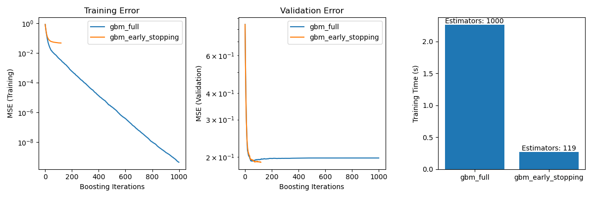
gbm_full 與 gbm_early_stopping 之間的訓練錯誤差異源於 gbm_early_stopping 將 validation_fraction 的訓練資料保留為內部驗證集的事實。提前停止是根據此內部驗證分數決定的。
摘要#
在我們使用加州房價資料集上的 GradientBoostingRegressor 模型的範例中,我們示範了提前停止的實際好處
防止過擬合:我們展示了驗證錯誤如何在某個點之後穩定或開始增加,表示模型更能推廣到未見的資料。這是透過在過擬合發生之前停止訓練過程來實現的。
提高訓練效率:我們比較了具有和不具有提前停止的模型的訓練時間。具有提前停止的模型在需要明顯較少的估計器的同時達成了可比較的準確度,從而縮短了訓練時間。
腳本的總執行時間:(0 分鐘 3.826 秒)
相關範例