注意
前往結尾以下載完整的範例程式碼。或透過 JupyterLite 或 Binder 在您的瀏覽器中執行此範例
使用樹集成進行特徵轉換#
將您的特徵轉換為更高維度、稀疏的空間。然後在這些特徵上訓練線性模型。
首先,在訓練集上擬合樹集成(完全隨機樹、隨機森林或梯度提升樹)。然後,將集成中每棵樹的每個葉子分配到新特徵空間中的固定任意特徵索引。然後,以獨熱方式編碼這些葉子索引。
每個樣本都會經歷集成中每棵樹的決策,並在每棵樹中結束於一個葉子。該樣本透過將這些葉子的特徵值設定為 1,將其他特徵值設定為 0 來進行編碼。
然後,產生的轉換器學習了資料的監督式、稀疏、高維類別嵌入。
# Authors: The scikit-learn developers
# SPDX-License-Identifier: BSD-3-Clause
首先,我們將建立一個大型資料集並將其分成三組
一組用於訓練稍後用作特徵工程轉換器的集成方法;
一組用於訓練線性模型;
一組用於測試線性模型。
以這種方式分割資料以避免透過洩漏資料而過擬合非常重要。
from sklearn.datasets import make_classification
from sklearn.model_selection import train_test_split

X, y = make_classification(n_samples=80_000, random_state=10)

X_full_train, X_test, y_full_train, y_test = train_test_split(
    X, y, test_size=0.5, random_state=10
)
X_train_ensemble, X_train_linear, y_train_ensemble, y_train_linear = train_test_split(
    X_full_train, y_full_train, test_size=0.5, random_state=10
)
對於每種集成方法,我們將使用 10 個估計器和最大深度 3 個層級。
n_estimators = 10
max_depth = 3
首先,我們將從在分離的訓練集上訓練隨機森林和梯度提升開始
from sklearn.ensemble import GradientBoostingClassifier, RandomForestClassifier

random_forest = RandomForestClassifier(
    n_estimators=n_estimators, max_depth=max_depth, random_state=10
)
random_forest.fit(X_train_ensemble, y_train_ensemble)

gradient_boosting = GradientBoostingClassifier(
    n_estimators=n_estimators, max_depth=max_depth, random_state=10
)
_ = gradient_boosting.fit(X_train_ensemble, y_train_ensemble)
請注意,從中間資料集開始 (n_samples >= 10_000),HistGradientBoostingClassifier 比 GradientBoostingClassifier 快得多,但本範例的情況並非如此。
RandomTreesEmbedding 是一種非監督式方法,因此不需要獨立訓練。
from sklearn.ensemble import RandomTreesEmbedding

random_tree_embedding = RandomTreesEmbedding(
    n_estimators=n_estimators, max_depth=max_depth, random_state=0
)
現在,我們將建立三個管道,這些管道將使用上述嵌入作為預處理階段。
隨機樹嵌入可以直接與邏輯迴歸管道化,因為它是標準的 scikit-learn 轉換器。
from sklearn.linear_model import LogisticRegression
from sklearn.pipeline import make_pipeline

rt_model = make_pipeline(random_tree_embedding, LogisticRegression(max_iter=1000))
rt_model.fit(X_train_linear, y_train_linear)
然後,我們可以使用邏輯迴歸將隨機森林或梯度提升管道化。但是,特徵轉換將透過呼叫方法 apply 進行。scikit-learn 中的管道預期呼叫 transform。因此,我們將對 apply 的呼叫包裝在 FunctionTransformer 中。
from sklearn.preprocessing import FunctionTransformer, OneHotEncoder


def rf_apply(X, model):
    return model.apply(X)


rf_leaves_yielder = FunctionTransformer(rf_apply, kw_args={"model": random_forest})

rf_model = make_pipeline(
    rf_leaves_yielder,
    OneHotEncoder(handle_unknown="ignore"),
    LogisticRegression(max_iter=1000),
)
rf_model.fit(X_train_linear, y_train_linear)
def gbdt_apply(X, model):
    return model.apply(X)[:, :, 0]


gbdt_leaves_yielder = FunctionTransformer(
    gbdt_apply, kw_args={"model": gradient_boosting}
)

gbdt_model = make_pipeline(
    gbdt_leaves_yielder,
    OneHotEncoder(handle_unknown="ignore"),
    LogisticRegression(max_iter=1000),
)
gbdt_model.fit(X_train_linear, y_train_linear)
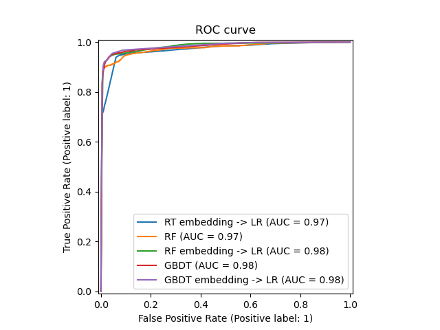
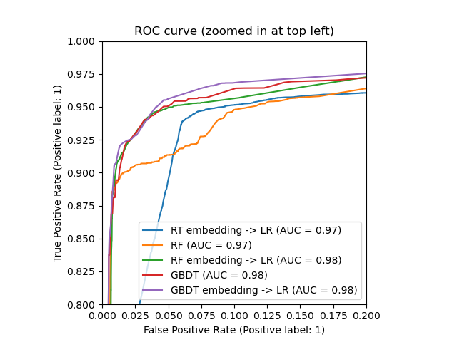
我們最終可以顯示所有模型不同的 ROC 曲線。
import matplotlib.pyplot as plt

from sklearn.metrics import RocCurveDisplay

_, ax = plt.subplots()

models = [
    ("RT embedding -> LR", rt_model),
    ("RF", random_forest),
    ("RF embedding -> LR", rf_model),
    ("GBDT", gradient_boosting),
    ("GBDT embedding -> LR", gbdt_model),
]

model_displays = {}
for name, pipeline in models:
    model_displays[name] = RocCurveDisplay.from_estimator(
        pipeline, X_test, y_test, ax=ax, name=name
    )
_ = ax.set_title("ROC curve")
_, ax = plt.subplots()
for name, pipeline in models:
    model_displays[name].plot(ax=ax)

ax.set_xlim(0, 0.2)
ax.set_ylim(0.8, 1)
_ = ax.set_title("ROC curve (zoomed in at top left)")
腳本的總執行時間:(0 分 3.002 秒)
相關範例