注意事項
前往結尾以下載完整範例程式碼。 或透過 JupyterLite 或 Binder 在您的瀏覽器中執行此範例
非負最小平方#
在此範例中,我們將線性模型擬合到迴歸係數上具有正約束的條件,並將估計的係數與經典線性迴歸進行比較。
# Authors: The scikit-learn developers
# SPDX-License-Identifier: BSD-3-Clause

import matplotlib.pyplot as plt
import numpy as np

from sklearn.metrics import r2_score
產生一些隨機資料
np.random.seed(42)

n_samples, n_features = 200, 50
X = np.random.randn(n_samples, n_features)
true_coef = 3 * np.random.randn(n_features)
# Threshold coefficients to render them non-negative
true_coef[true_coef < 0] = 0
y = np.dot(X, true_coef)

# Add some noise
y += 5 * np.random.normal(size=(n_samples,))
將資料分割為訓練集和測試集
from sklearn.model_selection import train_test_split

X_train, X_test, y_train, y_test = train_test_split(X, y, test_size=0.5)
擬合非負最小平方。
from sklearn.linear_model import LinearRegression

reg_nnls = LinearRegression(positive=True)
y_pred_nnls = reg_nnls.fit(X_train, y_train).predict(X_test)
r2_score_nnls = r2_score(y_test, y_pred_nnls)
print("NNLS R2 score", r2_score_nnls)
NNLS R2 score 0.8225220806196525
擬合 OLS。
reg_ols = LinearRegression()
y_pred_ols = reg_ols.fit(X_train, y_train).predict(X_test)
r2_score_ols = r2_score(y_test, y_pred_ols)
print("OLS R2 score", r2_score_ols)
OLS R2 score 0.7436926291700353
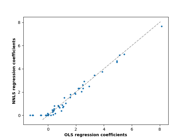
比較 OLS 和 NNLS 之間的迴歸係數,我們可以觀察到它們高度相關 (虛線是恆等關係),但非負約束會將某些係數縮小為 0。非負最小平方本質上會產生稀疏結果。
fig, ax = plt.subplots()
ax.plot(reg_ols.coef_, reg_nnls.coef_, linewidth=0, marker=".")

low_x, high_x = ax.get_xlim()
low_y, high_y = ax.get_ylim()
low = max(low_x, low_y)
high = min(high_x, high_y)
ax.plot([low, high], [low, high], ls="--", c=".3", alpha=0.5)
ax.set_xlabel("OLS regression coefficients", fontweight="bold")
ax.set_ylabel("NNLS regression coefficients", fontweight="bold")
Text(55.847222222222214, 0.5, 'NNLS regression coefficients')
腳本的總執行時間: (0 分鐘 0.068 秒)
相關範例