注意
跳到結尾下載完整的範例程式碼。或透過 JupyterLite 或 Binder 在您的瀏覽器中執行此範例
部分依賴性和個別條件期望圖#
部分依賴性圖顯示目標函數 [2] 與一組感興趣的特徵之間的依賴性,邊緣化所有其他特徵(補充特徵)的值。由於人類感知的限制,感興趣的特徵集合大小必須很小(通常為一個或兩個),因此它們通常在最重要的特徵中選擇。
同樣地,個別條件期望 (ICE) 圖 [3] 顯示目標函數與感興趣的特徵之間的依賴性。然而,與顯示感興趣特徵平均效果的部分依賴性圖不同,ICE 圖會視覺化預測對每個樣本的特徵的依賴性,每個樣本一條線。ICE 圖僅支援一個感興趣的特徵。
此範例說明如何從在自行車共享資料集上訓練的 MLPRegressor 和 HistGradientBoostingRegressor 取得部分依賴性和 ICE 圖。該範例的靈感來自 [1]。
# Authors: The scikit-learn developers
# SPDX-License-Identifier: BSD-3-Clause
自行車共享資料集預處理#
我們將使用自行車共享資料集。目標是使用天氣和季節資料以及日期時間資訊來預測自行車租賃數量。
from sklearn.datasets import fetch_openml

bikes = fetch_openml("Bike_Sharing_Demand", version=2, as_frame=True)
# Make an explicit copy to avoid "SettingWithCopyWarning" from pandas
X, y = bikes.data.copy(), bikes.target

# We use only a subset of the data to speed up the example.
X = X.iloc[::5, :]
y = y[::5]
特徵 "weather" 有一個特殊之處:"heavy_rain" 類別是一個罕見的類別。
X["weather"].value_counts()
weather
clear         2284
misty          904
rain           287
heavy_rain       1
Name: count, dtype: int64
由於這個罕見的類別,我們將其折疊為 "rain"。
X["weather"] = (
    X["weather"]
    .astype(object)
    .replace(to_replace="heavy_rain", value="rain")
    .astype("category")
)
我們現在更仔細地查看 "year" 特徵
X["year"].value_counts()
year
1    1747
0    1729
Name: count, dtype: int64
我們看到我們有兩年的資料。我們使用第一年來訓練模型,第二年來測試模型。
mask_training = X["year"] == 0.0
X = X.drop(columns=["year"])
X_train, y_train = X[mask_training], y[mask_training]
X_test, y_test = X[~mask_training], y[~mask_training]
我們可以檢查資料集資訊,看看我們是否有異質的資料類型。我們必須相應地預處理不同的欄。
X_train.info()
<class 'pandas.core.frame.DataFrame'>
Index: 1729 entries, 0 to 8640
Data columns (total 11 columns):
 #   Column      Non-Null Count  Dtype
---  ------      --------------  -----
 0   season      1729 non-null   category
 1   month       1729 non-null   int64
 2   hour        1729 non-null   int64
 3   holiday     1729 non-null   category
 4   weekday     1729 non-null   int64
 5   workingday  1729 non-null   category
 6   weather     1729 non-null   category
 7   temp        1729 non-null   float64
 8   feel_temp   1729 non-null   float64
 9   humidity    1729 non-null   float64
 10  windspeed   1729 non-null   float64
dtypes: category(4), float64(4), int64(3)
memory usage: 115.4 KB
根據先前的資訊,我們會將 category 欄視為名義類別特徵。此外,我們還會將日期和時間資訊視為類別特徵。
我們會手動定義包含數值和類別特徵的欄。
numerical_features = [
    "temp",
    "feel_temp",
    "humidity",
    "windspeed",
]
categorical_features = X_train.columns.drop(numerical_features)
在我們深入了解不同機器學習管道的預處理細節之前,我們將嘗試獲得一些關於資料集的額外直觀理解,這將有助於了解模型的統計效能和部分依賴性分析的結果。
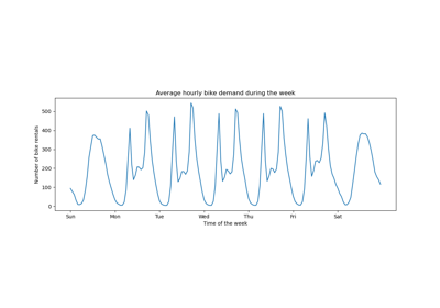
我們繪製按季節和年份分組的平均自行車租賃數量。
from itertools import product

import matplotlib.pyplot as plt
import numpy as np

days = ("Sun", "Mon", "Tue", "Wed", "Thu", "Fri", "Sat")
hours = tuple(range(24))
xticklabels = [f"{day}\n{hour}:00" for day, hour in product(days, hours)]
xtick_start, xtick_period = 6, 12

fig, axs = plt.subplots(nrows=2, figsize=(8, 6), sharey=True, sharex=True)
average_bike_rentals = bikes.frame.groupby(
    ["year", "season", "weekday", "hour"], observed=True
).mean(numeric_only=True)["count"]
for ax, (idx, df) in zip(axs, average_bike_rentals.groupby("year")):
    df.groupby("season", observed=True).plot(ax=ax, legend=True)

    # decorate the plot
    ax.set_xticks(
        np.linspace(
            start=xtick_start,
            stop=len(xticklabels),
            num=len(xticklabels) // xtick_period,
        )
    )
    ax.set_xticklabels(xticklabels[xtick_start::xtick_period])
    ax.set_xlabel("")
    ax.set_ylabel("Average number of bike rentals")
    ax.set_title(
        f"Bike rental for {'2010 (train set)' if idx == 0.0 else '2011 (test set)'}"
    )
    ax.set_ylim(0, 1_000)
    ax.set_xlim(0, len(xticklabels))
    ax.legend(loc=2)
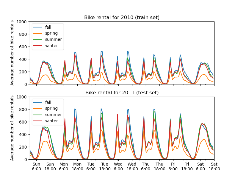
訓練集和測試集之間的第一個顯著差異是測試集中的自行車租賃數量較高。因此,取得低估自行車租賃數量的機器學習模型並不足為奇。我們還觀察到,春季的自行車租賃數量較少。此外,我們看到在工作日,大約早上 6-7 點和下午 5-6 點左右有一個特殊的模式,其中有一些自行車租賃高峰。我們可以記住這些不同的見解,並使用它們來理解部分依賴性圖。
機器學習模型的預處理器#
由於我們稍後會使用兩個不同的模型,一個 MLPRegressor 和一個 HistGradientBoostingRegressor,我們會建立兩個不同的預處理器,每個模型都有其專屬的預處理器。
神經網路模型的預處理器#
我們將使用 QuantileTransformer 來縮放數值特徵,並使用 OneHotEncoder 編碼類別特徵。
from sklearn.compose import ColumnTransformer
from sklearn.preprocessing import OneHotEncoder, QuantileTransformer

mlp_preprocessor = ColumnTransformer(
    transformers=[
        ("num", QuantileTransformer(n_quantiles=100), numerical_features),
        ("cat", OneHotEncoder(handle_unknown="ignore"), categorical_features),
    ]
)
mlp_preprocessor
梯度提升模型的前處理器#
對於梯度提升模型,我們將數值特徵保持原樣,僅使用 OrdinalEncoder 編碼類別特徵。
from sklearn.preprocessing import OrdinalEncoder

hgbdt_preprocessor = ColumnTransformer(
    transformers=[
        ("cat", OrdinalEncoder(), categorical_features),
        ("num", "passthrough", numerical_features),
    ],
    sparse_threshold=1,
    verbose_feature_names_out=False,
).set_output(transform="pandas")
hgbdt_preprocessor
使用不同模型的單向偏依性 (Partial Dependence)#
在本節中,我們將使用兩種不同的機器學習模型計算單向偏依性:(i) 多層感知器 (multi-layer perceptron) 和 (ii) 梯度提升模型。透過這兩個模型,我們將說明如何計算和解釋數值和類別特徵的偏依性圖 (Partial Dependence Plot, PDP) 和個別條件期望 (Individual Conditional Expectation, ICE)。
多層感知器#
讓我們擬合一個 MLPRegressor,並計算單變數偏依性圖。
from time import time

from sklearn.neural_network import MLPRegressor
from sklearn.pipeline import make_pipeline

print("Training MLPRegressor...")
tic = time()
mlp_model = make_pipeline(
    mlp_preprocessor,
    MLPRegressor(
        hidden_layer_sizes=(30, 15),
        learning_rate_init=0.01,
        early_stopping=True,
        random_state=0,
    ),
)
mlp_model.fit(X_train, y_train)
print(f"done in {time() - tic:.3f}s")
print(f"Test R2 score: {mlp_model.score(X_test, y_test):.2f}")
Training MLPRegressor...
done in 0.679s
Test R2 score: 0.61
我們使用專為神經網路建立的前處理器配置了一個 pipeline,並調整了神經網路的大小和學習率,以在訓練時間和測試集上的預測效能之間取得合理的平衡。
重要的是,這個表格資料集的特徵具有非常不同的動態範圍。神經網路往往對具有不同尺度的特徵非常敏感,而忘記預處理數值特徵會導致模型效能非常差。
透過更大的神經網路,有可能獲得更高的預測效能,但訓練成本也會顯著增加。
請注意,在繪製偏依性圖之前,檢查模型在測試集上的準確度是否足夠是很重要的,因為解釋給定特徵對預測效能不佳的模型的預測函數的影響沒有什麼意義。在這方面,我們的 MLP 模型表現相當不錯。
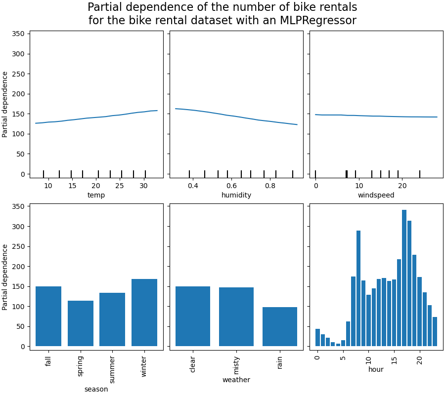
我們將繪製平均偏依性。
import matplotlib.pyplot as plt

from sklearn.inspection import PartialDependenceDisplay

common_params = {
    "subsample": 50,
    "n_jobs": 2,
    "grid_resolution": 20,
    "random_state": 0,
}

print("Computing partial dependence plots...")
features_info = {
    # features of interest
    "features": ["temp", "humidity", "windspeed", "season", "weather", "hour"],
    # type of partial dependence plot
    "kind": "average",
    # information regarding categorical features
    "categorical_features": categorical_features,
}
tic = time()
_, ax = plt.subplots(ncols=3, nrows=2, figsize=(9, 8), constrained_layout=True)
display = PartialDependenceDisplay.from_estimator(
    mlp_model,
    X_train,
    **features_info,
    ax=ax,
    **common_params,
)
print(f"done in {time() - tic:.3f}s")
_ = display.figure_.suptitle(
    (
        "Partial dependence of the number of bike rentals\n"
        "for the bike rental dataset with an MLPRegressor"
    ),
    fontsize=16,
)
Computing partial dependence plots...
done in 0.649s
梯度提升#
現在讓我們擬合一個 HistGradientBoostingRegressor,並計算相同特徵的偏依性。我們還使用專為此模型建立的特定前處理器。
from sklearn.ensemble import HistGradientBoostingRegressor

print("Training HistGradientBoostingRegressor...")
tic = time()
hgbdt_model = make_pipeline(
    hgbdt_preprocessor,
    HistGradientBoostingRegressor(
        categorical_features=categorical_features,
        random_state=0,
        max_iter=50,
    ),
)
hgbdt_model.fit(X_train, y_train)
print(f"done in {time() - tic:.3f}s")
print(f"Test R2 score: {hgbdt_model.score(X_test, y_test):.2f}")
Training HistGradientBoostingRegressor...
done in 0.128s
Test R2 score: 0.62
在這裡,我們使用了梯度提升模型的預設超參數,沒有進行任何預處理,因為基於樹的模型本質上對數值特徵的單調轉換具有穩健性。
請注意,在這個表格資料集上,梯度提升機 (Gradient Boosting Machines) 的訓練速度明顯快於神經網路,而且更準確。調整它們的超參數也明顯便宜得多(預設值通常效果很好,但神經網路通常不是這種情況)。
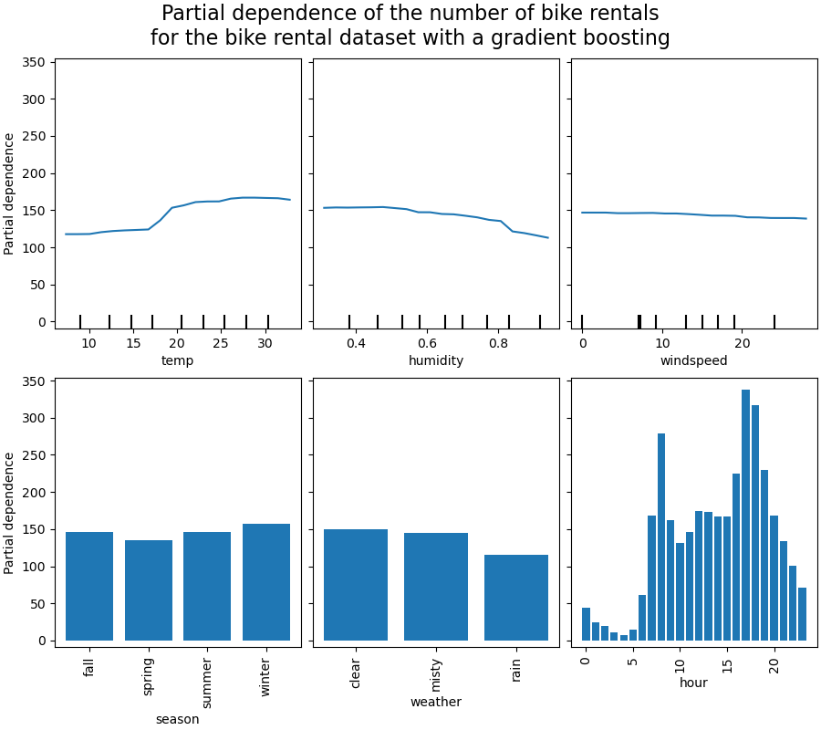
我們將繪製一些數值和類別特徵的偏依性。
print("Computing partial dependence plots...")
tic = time()
_, ax = plt.subplots(ncols=3, nrows=2, figsize=(9, 8), constrained_layout=True)
display = PartialDependenceDisplay.from_estimator(
    hgbdt_model,
    X_train,
    **features_info,
    ax=ax,
    **common_params,
)
print(f"done in {time() - tic:.3f}s")
_ = display.figure_.suptitle(
    (
        "Partial dependence of the number of bike rentals\n"
        "for the bike rental dataset with a gradient boosting"
    ),
    fontsize=16,
)
Computing partial dependence plots...
done in 1.218s
分析圖表#
我們將首先查看數值特徵的 PDP。對於這兩個模型,溫度 PDP 的總體趨勢是自行車租賃數量隨著溫度升高而增加。我們可以對濕度特徵進行類似的分析,但趨勢相反。當濕度增加時,自行車租賃數量會減少。最後,我們看到風速特徵的趨勢相同。對於這兩個模型,當風速增加時,自行車租賃數量會減少。我們還觀察到 MLPRegressor 的預測比 HistGradientBoostingRegressor 平滑得多。
現在,我們將查看類別特徵的偏依性圖。
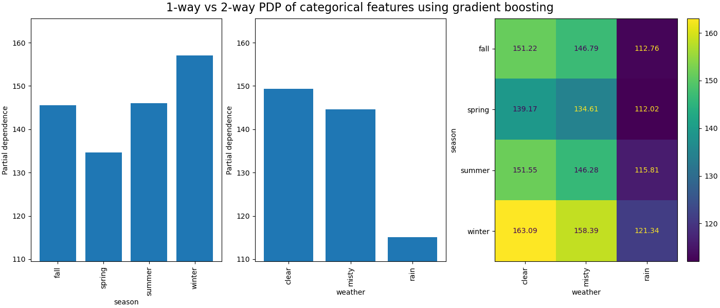
我們觀察到,對於 season 特徵,春季是最低的長條。對於 weather 特徵,rain 類別是最低的長條。關於 hour 特徵,我們看到早上 7 點和晚上 6 點左右有兩個高峰。這些發現與我們之前在資料集上觀察到的結果一致。
但是,值得注意的是,如果特徵相關,我們可能會產生毫無意義的合成樣本。
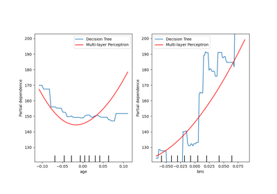
ICE vs. PDP#
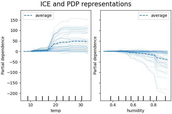
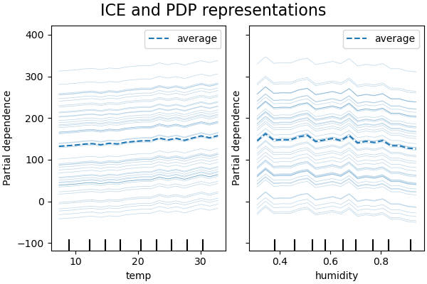
PDP 是特徵邊際效應的平均值。我們正在平均提供的集合中所有樣本的回應。因此,某些影響可能會被隱藏。在這方面,可以繪製每個單獨的回應。這種表示形式稱為個別效應圖 (Individual Effect Plot, ICE)。在下面的圖中,我們繪製了溫度和濕度特徵的 50 個隨機選擇的 ICE。
print("Computing partial dependence plots and individual conditional expectation...")
tic = time()
_, ax = plt.subplots(ncols=2, figsize=(6, 4), sharey=True, constrained_layout=True)

features_info = {
    "features": ["temp", "humidity"],
    "kind": "both",
    "centered": True,
}

display = PartialDependenceDisplay.from_estimator(
    hgbdt_model,
    X_train,
    **features_info,
    ax=ax,
    **common_params,
)
print(f"done in {time() - tic:.3f}s")
_ = display.figure_.suptitle("ICE and PDP representations", fontsize=16)
Computing partial dependence plots and individual conditional expectation...
done in 0.507s
我們看到,溫度特徵的 ICE 給了我們一些額外的資訊:一些 ICE 線是平坦的,而另一些則顯示當溫度高於攝氏 35 度時,依賴性會下降。我們觀察到濕度特徵的類似模式:當濕度高於 80% 時,某些 ICE 線會急劇下降。
並非所有 ICE 線都是平行的,這表示模型發現特徵之間存在交互作用。我們可以重複實驗,方法是限制梯度提升模型不使用特徵之間的任何交互作用,使用參數 interaction_cst
from sklearn.base import clone

interaction_cst = [[i] for i in range(X_train.shape[1])]
hgbdt_model_without_interactions = (
    clone(hgbdt_model)
    .set_params(histgradientboostingregressor__interaction_cst=interaction_cst)
    .fit(X_train, y_train)
)
print(f"Test R2 score: {hgbdt_model_without_interactions.score(X_test, y_test):.2f}")
Test R2 score: 0.38
_, ax = plt.subplots(ncols=2, figsize=(6, 4), sharey=True, constrained_layout=True)

features_info["centered"] = False
display = PartialDependenceDisplay.from_estimator(
    hgbdt_model_without_interactions,
    X_train,
    **features_info,
    ax=ax,
    **common_params,
)
_ = display.figure_.suptitle("ICE and PDP representations", fontsize=16)
2D 交互作用圖#
具有兩個感興趣特徵的 PDP 使我們能夠視覺化它們之間的交互作用。但是,ICE 無法以簡單的方式繪製,因此難以解釋。我們將展示 from_estimator 中可用的表示形式,即 2D 熱圖。
print("Computing partial dependence plots...")
features_info = {
    "features": ["temp", "humidity", ("temp", "humidity")],
    "kind": "average",
}
_, ax = plt.subplots(ncols=3, figsize=(10, 4), constrained_layout=True)
tic = time()
display = PartialDependenceDisplay.from_estimator(
    hgbdt_model,
    X_train,
    **features_info,
    ax=ax,
    **common_params,
)
print(f"done in {time() - tic:.3f}s")
_ = display.figure_.suptitle(
    "1-way vs 2-way of numerical PDP using gradient boosting", fontsize=16
)
Computing partial dependence plots...
done in 8.160s
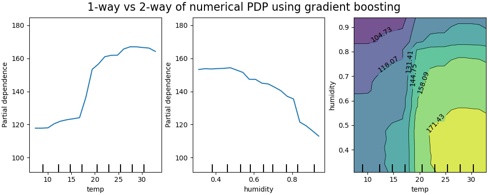
雙向偏依性圖顯示了自行車租賃數量對溫度和濕度聯合值的依賴性。我們清楚地看到這兩個特徵之間存在交互作用。對於高於攝氏 20 度的溫度,濕度對自行車租賃數量的影響似乎與溫度無關。
另一方面,對於低於攝氏 20 度的溫度,溫度和濕度都會持續影響自行車租賃數量。
此外,攝氏 20 度閾值的影響脊線的斜率非常依賴於濕度水平:在乾燥條件下,脊線很陡峭,但在濕度高於 70% 的潮濕條件下,脊線則平滑得多。
現在,我們將這些結果與針對限制為學習不依賴於這種非線性特徵交互作用的預測函數的模型計算的相同圖表進行比較。
print("Computing partial dependence plots...")
features_info = {
    "features": ["temp", "humidity", ("temp", "humidity")],
    "kind": "average",
}
_, ax = plt.subplots(ncols=3, figsize=(10, 4), constrained_layout=True)
tic = time()
display = PartialDependenceDisplay.from_estimator(
    hgbdt_model_without_interactions,
    X_train,
    **features_info,
    ax=ax,
    **common_params,
)
print(f"done in {time() - tic:.3f}s")
_ = display.figure_.suptitle(
    "1-way vs 2-way of numerical PDP using gradient boosting", fontsize=16
)
Computing partial dependence plots...
done in 7.703s
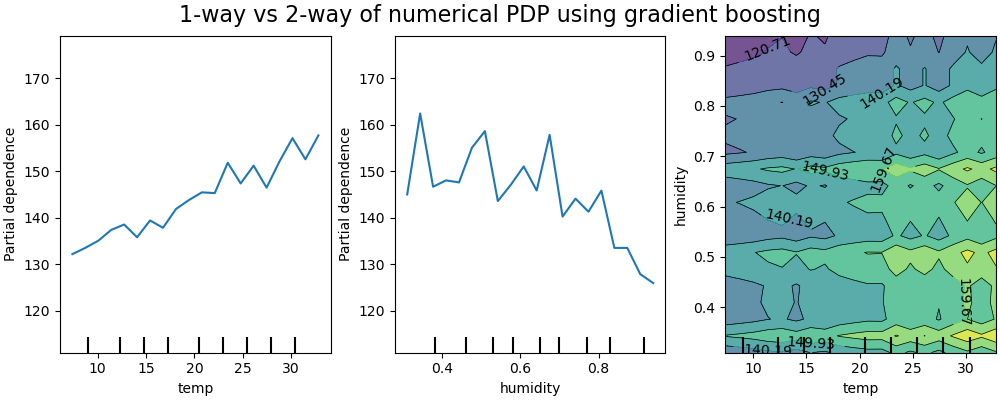
針對限制為不建模特徵交互作用的模型的一維偏依性圖顯示每個特徵的局部峰值,特別是對於「濕度」特徵。這些峰值可能反映了模型的行為退化,該模型試圖透過過度擬合特定的訓練點來彌補禁止的交互作用。請注意,此模型在測試集上測量的預測效能明顯低於原始未受限模型的預測效能。
另請注意,這些圖上可見的局部峰值數量取決於 PD 圖本身的網格解析度參數。
這些局部峰值導致一個有雜訊的網格 2D PD 圖。由於濕度特徵中的高頻振盪,很難判斷這些特徵之間是否存在交互作用。但是,可以清楚地看到,當溫度跨越 20 度邊界時觀察到的簡單交互作用效果對於此模型不再可見。
類別特徵之間的偏依性將提供離散表示形式,可以顯示為熱圖。例如,季節、天氣和目標之間的交互作用如下所示
print("Computing partial dependence plots...")
features_info = {
    "features": ["season", "weather", ("season", "weather")],
    "kind": "average",
    "categorical_features": categorical_features,
}
_, ax = plt.subplots(ncols=3, figsize=(14, 6), constrained_layout=True)
tic = time()
display = PartialDependenceDisplay.from_estimator(
    hgbdt_model,
    X_train,
    **features_info,
    ax=ax,
    **common_params,
)

print(f"done in {time() - tic:.3f}s")
_ = display.figure_.suptitle(
    "1-way vs 2-way PDP of categorical features using gradient boosting", fontsize=16
)
Computing partial dependence plots...
done in 0.732s
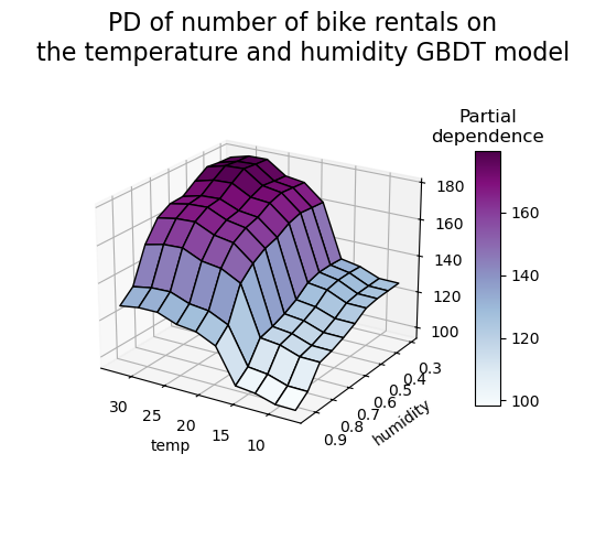
3D 表示法#
讓我們對 2 個特徵交互作用繪製相同的偏依性圖,這次是 3 維。
# unused but required import for doing 3d projections with matplotlib < 3.2
import mpl_toolkits.mplot3d  # noqa: F401
import numpy as np

from sklearn.inspection import partial_dependence

fig = plt.figure(figsize=(5.5, 5))

features = ("temp", "humidity")
pdp = partial_dependence(
    hgbdt_model, X_train, features=features, kind="average", grid_resolution=10
)
XX, YY = np.meshgrid(pdp["grid_values"][0], pdp["grid_values"][1])
Z = pdp.average[0].T
ax = fig.add_subplot(projection="3d")
fig.add_axes(ax)

surf = ax.plot_surface(XX, YY, Z, rstride=1, cstride=1, cmap=plt.cm.BuPu, edgecolor="k")
ax.set_xlabel(features[0])
ax.set_ylabel(features[1])
fig.suptitle(
    "PD of number of bike rentals on\nthe temperature and humidity GBDT model",
    fontsize=16,
)
# pretty init view
ax.view_init(elev=22, azim=122)
clb = plt.colorbar(surf, pad=0.08, shrink=0.6, aspect=10)
clb.ax.set_title("Partial\ndependence")
plt.show()
腳本的總執行時間:(0 分鐘 25.018 秒)
相關範例