注意
前往結尾以下載完整的範例程式碼。或透過 JupyterLite 或 Binder 在您的瀏覽器中執行此範例
用於時間序列預測的滯後特徵#
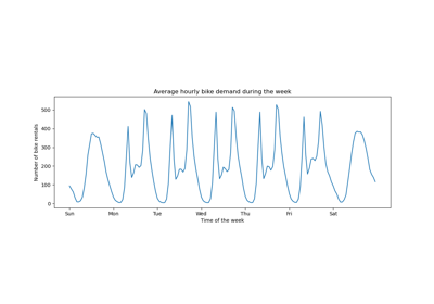
此範例展示如何將 Polars 工程化的滯後特徵用於 HistGradientBoostingRegressor 在自行車共享需求資料集上進行時間序列預測。
請參閱時間相關特徵工程範例,以了解此資料集的一些資料探索和週期性特徵工程的示範。
# Authors: The scikit-learn developers
# SPDX-License-Identifier: BSD-3-Clause
分析自行車共享需求資料集#
我們首先從 OpenML 儲存庫載入資料作為原始 parquet 檔案,以說明如何使用任意 parquet 檔案,而不是將此步驟隱藏在便利工具(例如 sklearn.datasets.fetch_openml)中。
parquet 檔案的 URL 可以在 openml.org 上 ID 為 44063 的自行車共享需求資料集的 JSON 描述中找到 (https://openml.org/search?type=data&status=active&id=44063)。
同時提供檔案的 sha256 雜湊值,以確保下載檔案的完整性。
import numpy as np
import polars as pl

from sklearn.datasets import fetch_file

pl.Config.set_fmt_str_lengths(20)

bike_sharing_data_file = fetch_file(
    "https://openml1.win.tue.nl/datasets/0004/44063/dataset_44063.pq",
    sha256="d120af76829af0d256338dc6dd4be5df4fd1f35bf3a283cab66a51c1c6abd06a",
)
bike_sharing_data_file
PosixPath('/home/circleci/scikit_learn_data/openml1.win.tue.nl/datasets_0004_44063/dataset_44063.pq')
我們使用 Polars 載入 parquet 檔案進行特徵工程。Polars 會自動快取在多個運算式中重複使用的通用子運算式(如下面的 pl.col("count").shift(1))。請參閱 https://docs.pola.rs/user-guide/lazy/optimizations/ 以取得更多資訊。
df = pl.read_parquet(bike_sharing_data_file)
接下來,我們來看一下資料集的統計摘要,以便更好地了解我們正在處理的資料。
import polars.selectors as cs

summary = df.select(cs.numeric()).describe()
summary
讓我們看看資料集中存在的 "秋季"、"春季"、"夏季" 和 "冬季" 季節的計數,以確認它們是否平衡。
import matplotlib.pyplot as plt

df["season"].value_counts()
產生 Polars 工程化的滯後特徵#
讓我們考慮預測過去需求給定的小時需求的問題。由於需求是一個連續變數,因此可以直觀地使用任何迴歸模型。然而,我們沒有通常的 (X_train, y_train) 資料集。相反,我們只有按時間順序組織的 y_train 需求資料。
lagged_df = df.select(
    "count",
    *[pl.col("count").shift(i).alias(f"lagged_count_{i}h") for i in [1, 2, 3]],
    lagged_count_1d=pl.col("count").shift(24),
    lagged_count_1d_1h=pl.col("count").shift(24 + 1),
    lagged_count_7d=pl.col("count").shift(7 * 24),
    lagged_count_7d_1h=pl.col("count").shift(7 * 24 + 1),
    lagged_mean_24h=pl.col("count").shift(1).rolling_mean(24),
    lagged_max_24h=pl.col("count").shift(1).rolling_max(24),
    lagged_min_24h=pl.col("count").shift(1).rolling_min(24),
    lagged_mean_7d=pl.col("count").shift(1).rolling_mean(7 * 24),
    lagged_max_7d=pl.col("count").shift(1).rolling_max(7 * 24),
    lagged_min_7d=pl.col("count").shift(1).rolling_min(7 * 24),
)
lagged_df.tail(10)
但是要注意,第一行有未定義的值,因為它們自己的過去是未知的。這取決於我們使用了多少滯後
lagged_df.head(10)
我們現在可以將滯後特徵分為一個矩陣 X,並將目標變數(要預測的計數)分為相同第一個維度的陣列 y。
lagged_df = lagged_df.drop_nulls()
X = lagged_df.drop("count")
y = lagged_df["count"]
print("X shape: {}\ny shape: {}".format(X.shape, y.shape))
X shape: (17210, 13)
y shape: (17210,)
對下一小時自行車需求迴歸的樸素評估#
讓我們隨機分割我們的表格化資料集,以訓練梯度提升迴歸樹 (GBRT) 模型,並使用平均絕對百分比誤差 (MAPE) 對其進行評估。如果我們的模型旨在進行預測(即,從過去的資料預測未來的資料),我們不應使用晚於測試資料的訓練資料。在時間序列機器學習中,“i.i.d”(獨立且均勻分佈)假設不成立,因為資料點不是獨立的,並且具有時間關係。
from sklearn.ensemble import HistGradientBoostingRegressor
from sklearn.model_selection import train_test_split

X_train, X_test, y_train, y_test = train_test_split(
    X, y, test_size=0.2, random_state=42
)

model = HistGradientBoostingRegressor().fit(X_train, y_train)
查看模型的效能。
from sklearn.metrics import mean_absolute_percentage_error

y_pred = model.predict(X_test)
mean_absolute_percentage_error(y_test, y_pred)
0.3889873516666431
適當的下一小時預測評估#
讓我們使用適當的評估分割策略,該策略會考慮資料集的時間結構,以評估我們的模型預測未來資料點的能力(避免從訓練集中的滯後特徵讀取值而作弊)。
from sklearn.model_selection import TimeSeriesSplit

ts_cv = TimeSeriesSplit(
    n_splits=3,  # to keep the notebook fast enough on common laptops
    gap=48,  # 2 days data gap between train and test
    max_train_size=10000,  # keep train sets of comparable sizes
    test_size=3000,  # for 2 or 3 digits of precision in scores
)
all_splits = list(ts_cv.split(X, y))
訓練模型並根據 MAPE 評估其效能。
train_idx, test_idx = all_splits[0]
X_train, X_test = X[train_idx, :], X[test_idx, :]
y_train, y_test = y[train_idx], y[test_idx]

model = HistGradientBoostingRegressor().fit(X_train, y_train)
y_pred = model.predict(X_test)
mean_absolute_percentage_error(y_test, y_pred)
0.44300751539296973
透過隨機訓練測試分割測量的泛化誤差過於樂觀。透過時間分割的泛化可能更能代表迴歸模型的真實效能。讓我們用適當的交叉驗證來評估這種誤差評估的變異性
from sklearn.model_selection import cross_val_score

cv_mape_scores = -cross_val_score(
    model, X, y, cv=ts_cv, scoring="neg_mean_absolute_percentage_error"
)
cv_mape_scores
array([0.44300752, 0.27772182, 0.3697178 ])
分割之間的變異性相當大!在實際情況下,建議使用更多分割來更好地評估變異性。從現在起,讓我們報告平均 CV 分數及其標準差。
print(f"CV MAPE: {cv_mape_scores.mean():.3f} ± {cv_mape_scores.std():.3f}")
CV MAPE: 0.363 ± 0.068
我們可以計算多種評估指標和損失函數的組合,這些組合在下面報告。
from collections import defaultdict

from sklearn.metrics import (
    make_scorer,
    mean_absolute_error,
    mean_pinball_loss,
    root_mean_squared_error,
)
from sklearn.model_selection import cross_validate


def consolidate_scores(cv_results, scores, metric):
    if metric == "MAPE":
        scores[metric].append(f"{value.mean():.2f} ± {value.std():.2f}")
    else:
        scores[metric].append(f"{value.mean():.1f} ± {value.std():.1f}")

    return scores


scoring = {
    "MAPE": make_scorer(mean_absolute_percentage_error),
    "RMSE": make_scorer(root_mean_squared_error),
    "MAE": make_scorer(mean_absolute_error),
    "pinball_loss_05": make_scorer(mean_pinball_loss, alpha=0.05),
    "pinball_loss_50": make_scorer(mean_pinball_loss, alpha=0.50),
    "pinball_loss_95": make_scorer(mean_pinball_loss, alpha=0.95),
}
loss_functions = ["squared_error", "poisson", "absolute_error"]
scores = defaultdict(list)
for loss_func in loss_functions:
    model = HistGradientBoostingRegressor(loss=loss_func)
    cv_results = cross_validate(
        model,
        X,
        y,
        cv=ts_cv,
        scoring=scoring,
        n_jobs=2,
    )
    time = cv_results["fit_time"]
    scores["loss"].append(loss_func)
    scores["fit_time"].append(f"{time.mean():.2f} ± {time.std():.2f} s")

    for key, value in cv_results.items():
        if key.startswith("test_"):
            metric = key.split("test_")[1]
            scores = consolidate_scores(cv_results, scores, metric)
透過分位數迴歸建模預測不確定性#
與最小二乘和 Poisson 損失所做的建模 \(Y|X\) 分佈的期望值不同,可以嘗試估計條件分佈的分位數。
\(Y|X=x_i\) 對於給定的資料點 \(x_i\) 預計是一個隨機變數,因為我們預計租賃次數無法根據特徵 100% 準確預測。它可能會受到其他變數的影響,而這些變數未被現有的滯後特徵正確捕捉。例如,在接下來的一個小時內是否會下雨無法完全從過去幾小時的自行車租賃資料中預測。這就是我們所謂的偶然不確定性。
分位數迴歸可以在不對其形狀做出強烈假設的情況下,更精確地描述該分佈。
quantile_list = [0.05, 0.5, 0.95]

for quantile in quantile_list:
    model = HistGradientBoostingRegressor(loss="quantile", quantile=quantile)
    cv_results = cross_validate(
        model,
        X,
        y,
        cv=ts_cv,
        scoring=scoring,
        n_jobs=2,
    )
    time = cv_results["fit_time"]
    scores["fit_time"].append(f"{time.mean():.2f} ± {time.std():.2f} s")

    scores["loss"].append(f"quantile {int(quantile*100)}")
    for key, value in cv_results.items():
        if key.startswith("test_"):
            metric = key.split("test_")[1]
            scores = consolidate_scores(cv_results, scores, metric)

scores_df = pl.DataFrame(scores)
scores_df
讓我們看看最小化每個指標的損失。
def min_arg(col):
    col_split = pl.col(col).str.split(" ")
    return pl.arg_sort_by(
        col_split.list.get(0).cast(pl.Float64),
        col_split.list.get(2).cast(pl.Float64),
    ).first()


scores_df.select(
    pl.col("loss").get(min_arg(col_name)).alias(col_name)
    for col_name in scores_df.columns
    if col_name != "loss"
)
即使由於數據集的變異性導致分數分佈重疊,但當 loss="squared_error" 時,平均 RMSE 確實較低,而當 loss="absolute_error" 時,平均 MAPE 較低,正如預期的那樣。對於分位數 5 和 95 的平均 Pinball 損失也是如此。對應於 50 分位數損失的分數與最小化其他損失函數獲得的分數重疊,MAE 的情況也是如此。
對預測的質化觀察#
我們現在可以視覺化模型在第 5 個百分位數、中位數和第 95 個百分位數方面的性能
all_splits = list(ts_cv.split(X, y))
train_idx, test_idx = all_splits[0]

X_train, X_test = X[train_idx, :], X[test_idx, :]
y_train, y_test = y[train_idx], y[test_idx]

max_iter = 50
gbrt_mean_poisson = HistGradientBoostingRegressor(loss="poisson", max_iter=max_iter)
gbrt_mean_poisson.fit(X_train, y_train)
mean_predictions = gbrt_mean_poisson.predict(X_test)

gbrt_median = HistGradientBoostingRegressor(
    loss="quantile", quantile=0.5, max_iter=max_iter
)
gbrt_median.fit(X_train, y_train)
median_predictions = gbrt_median.predict(X_test)

gbrt_percentile_5 = HistGradientBoostingRegressor(
    loss="quantile", quantile=0.05, max_iter=max_iter
)
gbrt_percentile_5.fit(X_train, y_train)
percentile_5_predictions = gbrt_percentile_5.predict(X_test)

gbrt_percentile_95 = HistGradientBoostingRegressor(
    loss="quantile", quantile=0.95, max_iter=max_iter
)
gbrt_percentile_95.fit(X_train, y_train)
percentile_95_predictions = gbrt_percentile_95.predict(X_test)
我們現在可以看看迴歸模型所做的預測
last_hours = slice(-96, None)
fig, ax = plt.subplots(figsize=(15, 7))
plt.title("Predictions by regression models")
ax.plot(
    y_test[last_hours],
    "x-",
    alpha=0.2,
    label="Actual demand",
    color="black",
)
ax.plot(
    median_predictions[last_hours],
    "^-",
    label="GBRT median",
)
ax.plot(
    mean_predictions[last_hours],
    "x-",
    label="GBRT mean (Poisson)",
)
ax.fill_between(
    np.arange(96),
    percentile_5_predictions[last_hours],
    percentile_95_predictions[last_hours],
    alpha=0.3,
    label="GBRT 90% interval",
)
_ = ax.legend()
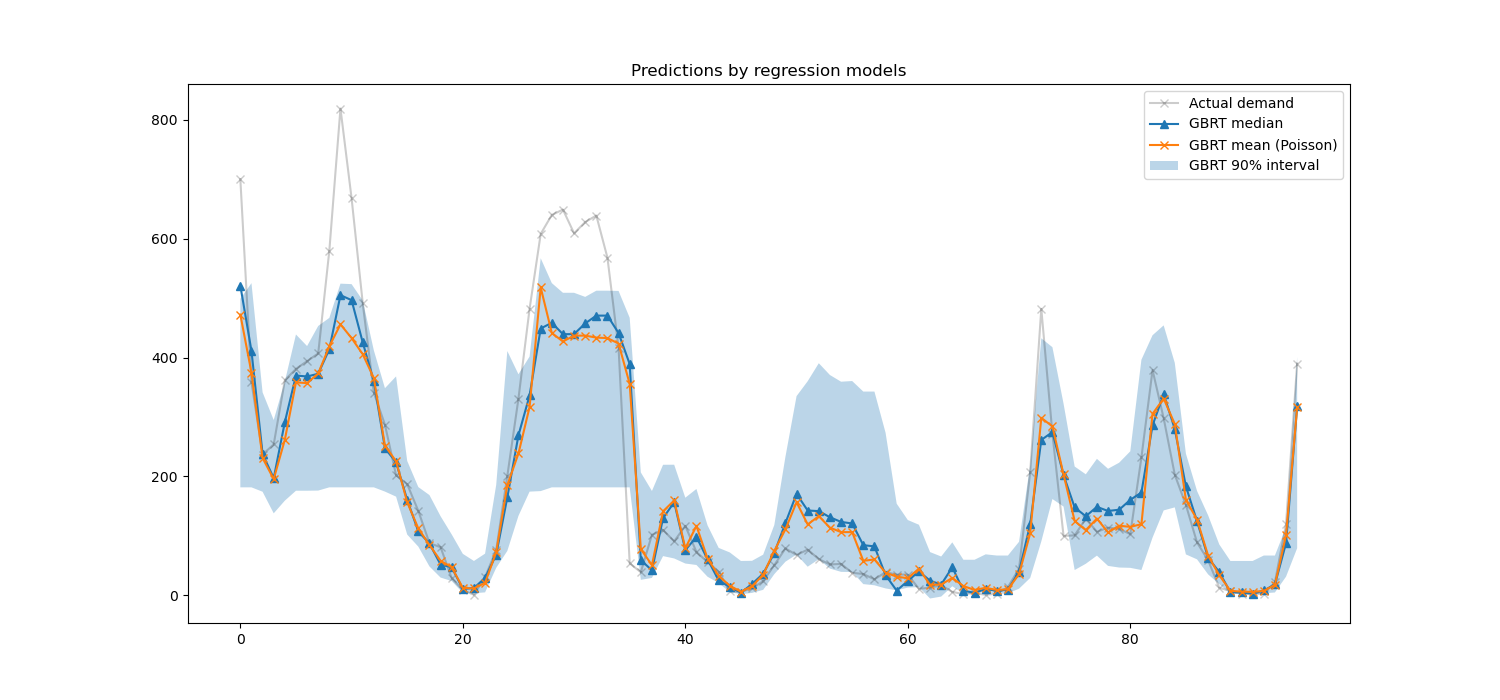
在這裡,值得注意的是,5% 和 95% 百分位數估計值之間的藍色區域的寬度隨著一天中的時間而變化
在晚上,藍色帶較窄:這對模型非常確定自行車租賃的數量將很少。此外,這些似乎是正確的,因為實際需求保持在藍色帶內。
白天,藍色帶較寬:不確定性增加,可能是因為天氣的變化可能產生非常大的影響,尤其是在週末。
我們也可以看到,在平日,通勤模式在 5% 和 95% 的估計值中仍然可見。
最後,預計有 10% 的時間,實際需求不會介於 5% 和 95% 的百分位數估計值之間。在這個測試範圍內,實際需求似乎更高,尤其是在高峰時段。這可能表明我們的 95% 百分位數估計值低估了需求峰值。這可以通過計算經驗覆蓋率數字來定量確認,如 信賴區間的校準 中所做的那樣。
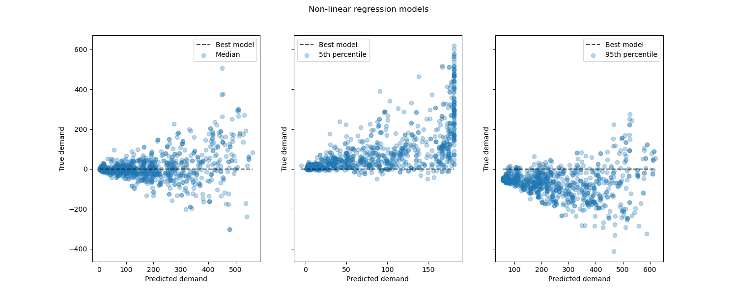
查看非線性迴歸模型相對於最佳模型的表現
from sklearn.metrics import PredictionErrorDisplay

fig, axes = plt.subplots(ncols=3, figsize=(15, 6), sharey=True)
fig.suptitle("Non-linear regression models")
predictions = [
    median_predictions,
    percentile_5_predictions,
    percentile_95_predictions,
]
labels = [
    "Median",
    "5th percentile",
    "95th percentile",
]
for ax, pred, label in zip(axes, predictions, labels):
    PredictionErrorDisplay.from_predictions(
        y_true=y_test,
        y_pred=pred,
        kind="residual_vs_predicted",
        scatter_kwargs={"alpha": 0.3},
        ax=ax,
    )
    ax.set(xlabel="Predicted demand", ylabel="True demand")
    ax.legend(["Best model", label])

plt.show()
結論#
通過這個範例,我們探索了使用滯後特徵的時間序列預測。我們將樸素迴歸(使用標準化的 train_test_split)與使用 TimeSeriesSplit 的正確時間序列評估策略進行了比較。我們觀察到,使用 train_test_split 訓練的模型,其 shuffle 的預設值設定為 True,產生了過於樂觀的平均絕對百分比誤差 (MAPE)。基於時間的分割所產生的結果更好地代表了我們的時間序列迴歸模型的效能。我們也通過分位數迴歸分析了我們模型的預測不確定性。使用 loss="quantile" 基於第 5 和 95 個百分位數的預測,為我們提供了對我們的時間序列迴歸模型所做預測的不確定性的定量估計。不確定性估計也可以使用 MAPIE 執行,它提供了基於近期對符合性預測方法的研究的實現,並同時估計了隨機不確定性和認知不確定性。此外,sktime 提供的功能可用於擴展 scikit-learn 估計器,方法是利用遞迴時間序列預測,這使得能夠動態預測未來值。
腳本的總執行時間:(0 分鐘 9.974 秒)
相關範例