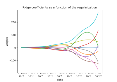
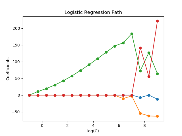
L1 邏輯迴歸的正規化路徑#

在從 Iris 資料集衍生的二元分類問題上訓練 l1 懲罰邏輯迴歸模型。

這些模型從最強的正規化到最弱的正規化依序排列。模型的 4 個係數被收集並繪製為「正規化路徑」：在圖的左側（強正規化器），所有係數都正好為 0。當正規化逐漸放鬆時，係數可以一個接一個地獲得非零值。

這裡我們選擇 liblinear 解算器，因為它可以有效地針對具有非平滑、稀疏誘導 l1 懲罰的邏輯迴歸損失進行最佳化。

另請注意，我們為容差設定了較低的值，以確保模型在收集係數之前已收斂。

我們還使用 warm_start=True，這表示模型的係數會被重複使用來初始化下一個模型擬合，以加速完整路徑的計算。

# Authors: The scikit-learn developers
# SPDX-License-Identifier: BSD-3-Clause

載入資料#

from sklearn import datasets

iris = datasets.load_iris()
X = iris.data
y = iris.target

X = X[y != 2]
y = y[y != 2]

X /= X.max()  # Normalize X to speed-up convergence

計算正規化路徑#

import numpy as np

from sklearn import linear_model
from sklearn.svm import l1_min_c

cs = l1_min_c(X, y, loss="log") * np.logspace(0, 10, 16)

clf = linear_model.LogisticRegression(
    penalty="l1",
    solver="liblinear",
    tol=1e-6,
    max_iter=int(1e6),
    warm_start=True,
    intercept_scaling=10000.0,
)
coefs_ = []
for c in cs:
    clf.set_params(C=c)
    clf.fit(X, y)
    coefs_.append(clf.coef_.ravel().copy())

coefs_ = np.array(coefs_)

繪製正規化路徑#

import matplotlib.pyplot as plt

plt.plot(np.log10(cs), coefs_, marker="o")
ymin, ymax = plt.ylim()
plt.xlabel("log(C)")
plt.ylabel("Coefficients")
plt.title("Logistic Regression Path")
plt.axis("tight")
plt.show()