混淆矩陣

混淆矩陣使用範例，評估分類器在虹膜資料集上的輸出品質。對角線元素表示預測標籤等於真實標籤的點數，而非對角線元素是分類器錯誤標記的點數。混淆矩陣的對角線值越高越好，表示許多正確的預測。

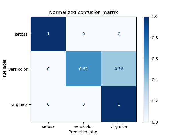
這些圖顯示了使用和不使用類別支援大小（每個類別中的元素數量）正規化的混淆矩陣。這種正規化在類別不平衡的情況下很有趣，可以更視覺化地解釋哪個類別被錯誤分類。

這裡的結果不如預期的好，因為我們選擇的正規化參數 C 不是最好的。在實際應用中，此參數通常使用 調整估計器的超參數 來選擇。

• 
• 

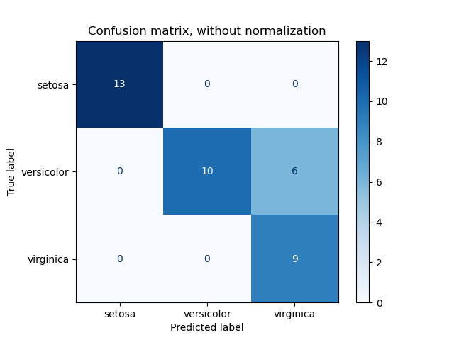
Confusion matrix, without normalization
[[13  0  0]
 [ 0 10  6]
 [ 0  0  9]]
Normalized confusion matrix
[[1.   0.   0.  ]
 [0.   0.62 0.38]
 [0.   0.   1.  ]]

# Authors: The scikit-learn developers
# SPDX-License-Identifier: BSD-3-Clause

import matplotlib.pyplot as plt
import numpy as np

from sklearn import datasets, svm
from sklearn.metrics import ConfusionMatrixDisplay
from sklearn.model_selection import train_test_split

# import some data to play with
iris = datasets.load_iris()
X = iris.data
y = iris.target
class_names = iris.target_names

# Split the data into a training set and a test set
X_train, X_test, y_train, y_test = train_test_split(X, y, random_state=0)

# Run classifier, using a model that is too regularized (C too low) to see
# the impact on the results
classifier = svm.SVC(kernel="linear", C=0.01).fit(X_train, y_train)

np.set_printoptions(precision=2)

# Plot non-normalized confusion matrix
titles_options = [
    ("Confusion matrix, without normalization", None),
    ("Normalized confusion matrix", "true"),
]
for title, normalize in titles_options:
    disp = ConfusionMatrixDisplay.from_estimator(
        classifier,
        X_test,
        y_test,
        display_labels=class_names,
        cmap=plt.cm.Blues,
        normalize=normalize,
    )
    disp.ax_.set_title(title)

    print(title)
    print(disp.confusion_matrix)

plt.show()

相關範例

辨識手寫數字

辨識手寫數字

鳶尾花資料集上的主成分分析 (PCA)

鳶尾花資料集上的主成分分析 (PCA)

最近鄰居分類

最近鄰居分類

在虹膜資料集中繪製不同的 SVM 分類器

在虹膜資料集中繪製不同的 SVM 分類器