改變自訓練閾值的影響#

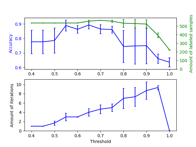
此範例說明自訓練中不同閾值的影響。載入 breast_cancer 資料集，並刪除標籤，使 569 個樣本中只有 50 個具有標籤。使用不同的閾值，將 SelfTrainingClassifier 擬合在此資料集上。

上面的圖表顯示分類器在擬合結束時可用的已標記樣本數量，以及分類器的準確性。下面的圖表顯示樣本被標記的最後一次迭代。所有值都經過 3 折交叉驗證。

在低閾值（在 [0.4, 0.5] 中）下，分類器從以低置信度標記的樣本中學習。這些低置信度樣本可能具有不正確的預測標籤，因此，擬合這些不正確的標籤會產生較差的準確性。請注意，分類器會標記幾乎所有樣本，並且僅需一次迭代。

對於非常高的閾值（在 [0.9, 1) 中），我們觀察到分類器不會擴充其資料集（自我標記的樣本數量為 0）。因此，使用 0.9999 閾值實現的準確性與普通監督分類器實現的準確性相同。

最佳準確性介於這兩個極端之間，閾值約為 0.7。

# Authors: The scikit-learn developers
# SPDX-License-Identifier: BSD-3-Clause

import matplotlib.pyplot as plt
import numpy as np

from sklearn import datasets
from sklearn.metrics import accuracy_score
from sklearn.model_selection import StratifiedKFold
from sklearn.semi_supervised import SelfTrainingClassifier
from sklearn.svm import SVC
from sklearn.utils import shuffle

n_splits = 3

X, y = datasets.load_breast_cancer(return_X_y=True)
X, y = shuffle(X, y, random_state=42)
y_true = y.copy()
y[50:] = -1
total_samples = y.shape[0]

base_classifier = SVC(probability=True, gamma=0.001, random_state=42)

x_values = np.arange(0.4, 1.05, 0.05)
x_values = np.append(x_values, 0.99999)
scores = np.empty((x_values.shape[0], n_splits))
amount_labeled = np.empty((x_values.shape[0], n_splits))
amount_iterations = np.empty((x_values.shape[0], n_splits))

for i, threshold in enumerate(x_values):
    self_training_clf = SelfTrainingClassifier(base_classifier, threshold=threshold)

    # We need manual cross validation so that we don't treat -1 as a separate
    # class when computing accuracy
    skfolds = StratifiedKFold(n_splits=n_splits)
    for fold, (train_index, test_index) in enumerate(skfolds.split(X, y)):
        X_train = X[train_index]
        y_train = y[train_index]
        X_test = X[test_index]
        y_test = y[test_index]
        y_test_true = y_true[test_index]

        self_training_clf.fit(X_train, y_train)

        # The amount of labeled samples that at the end of fitting
        amount_labeled[i, fold] = (
            total_samples
            - np.unique(self_training_clf.labeled_iter_, return_counts=True)[1][0]
        )
        # The last iteration the classifier labeled a sample in
        amount_iterations[i, fold] = np.max(self_training_clf.labeled_iter_)

        y_pred = self_training_clf.predict(X_test)
        scores[i, fold] = accuracy_score(y_test_true, y_pred)


ax1 = plt.subplot(211)
ax1.errorbar(
    x_values, scores.mean(axis=1), yerr=scores.std(axis=1), capsize=2, color="b"
)
ax1.set_ylabel("Accuracy", color="b")
ax1.tick_params("y", colors="b")

ax2 = ax1.twinx()
ax2.errorbar(
    x_values,
    amount_labeled.mean(axis=1),
    yerr=amount_labeled.std(axis=1),
    capsize=2,
    color="g",
)
ax2.set_ylim(bottom=0)
ax2.set_ylabel("Amount of labeled samples", color="g")
ax2.tick_params("y", colors="g")

ax3 = plt.subplot(212, sharex=ax1)
ax3.errorbar(
    x_values,
    amount_iterations.mean(axis=1),
    yerr=amount_iterations.std(axis=1),
    capsize=2,
    color="b",
)
ax3.set_ylim(bottom=0)
ax3.set_ylabel("Amount of iterations")
ax3.set_xlabel("Threshold")

plt.show()