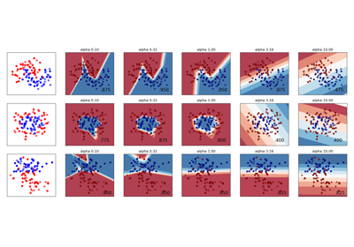
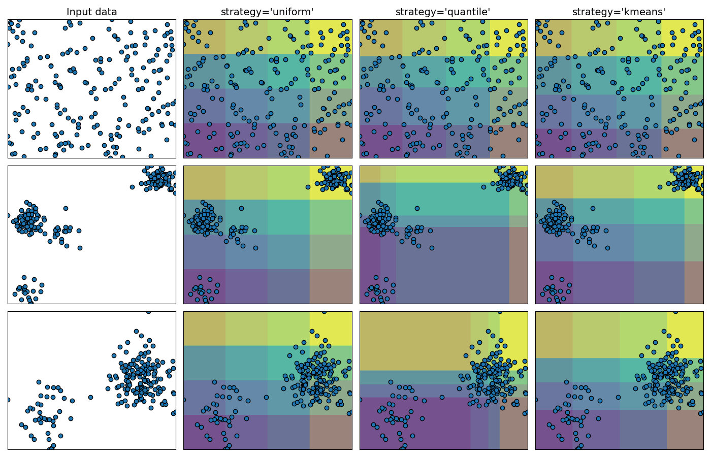
示範 KBinsDiscretizer 的不同策略#

此範例呈現 KBinsDiscretizer 中實作的不同策略

「uniform」：離散化在每個特徵中是均勻的，這表示箱寬在每個維度中是恆定的。
「quantile」：離散化是在分位數值上完成的，這表示每個箱子具有大約相同數量的樣本。
「kmeans」：離散化是基於 KMeans 群集程序的質心。

此圖顯示離散化編碼為常數的區域。

Input data, strategy='uniform', strategy='quantile', strategy='kmeans'

# Authors: The scikit-learn developers
# SPDX-License-Identifier: BSD-3-Clause

import matplotlib.pyplot as plt
import numpy as np

from sklearn.datasets import make_blobs
from sklearn.preprocessing import KBinsDiscretizer

strategies = ["uniform", "quantile", "kmeans"]

n_samples = 200
centers_0 = np.array([[0, 0], [0, 5], [2, 4], [8, 8]])
centers_1 = np.array([[0, 0], [3, 1]])

# construct the datasets
random_state = 42
X_list = [
    np.random.RandomState(random_state).uniform(-3, 3, size=(n_samples, 2)),
    make_blobs(
        n_samples=[
            n_samples // 10,
            n_samples * 4 // 10,
            n_samples // 10,
            n_samples * 4 // 10,
        ],
        cluster_std=0.5,
        centers=centers_0,
        random_state=random_state,
    )[0],
    make_blobs(
        n_samples=[n_samples // 5, n_samples * 4 // 5],
        cluster_std=0.5,
        centers=centers_1,
        random_state=random_state,
    )[0],
]

figure = plt.figure(figsize=(14, 9))
i = 1
for ds_cnt, X in enumerate(X_list):
    ax = plt.subplot(len(X_list), len(strategies) + 1, i)
    ax.scatter(X[:, 0], X[:, 1], edgecolors="k")
    if ds_cnt == 0:
        ax.set_title("Input data", size=14)

    xx, yy = np.meshgrid(
        np.linspace(X[:, 0].min(), X[:, 0].max(), 300),
        np.linspace(X[:, 1].min(), X[:, 1].max(), 300),
    )
    grid = np.c_[xx.ravel(), yy.ravel()]

    ax.set_xlim(xx.min(), xx.max())
    ax.set_ylim(yy.min(), yy.max())
    ax.set_xticks(())
    ax.set_yticks(())

    i += 1
    # transform the dataset with KBinsDiscretizer
    for strategy in strategies:
        enc = KBinsDiscretizer(n_bins=4, encode="ordinal", strategy=strategy)
        enc.fit(X)
        grid_encoded = enc.transform(grid)

        ax = plt.subplot(len(X_list), len(strategies) + 1, i)

        # horizontal stripes
        horizontal = grid_encoded[:, 0].reshape(xx.shape)
        ax.contourf(xx, yy, horizontal, alpha=0.5)
        # vertical stripes
        vertical = grid_encoded[:, 1].reshape(xx.shape)
        ax.contourf(xx, yy, vertical, alpha=0.5)

        ax.scatter(X[:, 0], X[:, 1], edgecolors="k")
        ax.set_xlim(xx.min(), xx.max())
        ax.set_ylim(yy.min(), yy.max())
        ax.set_xticks(())
        ax.set_yticks(())
        if ds_cnt == 0:
            ax.set_title("strategy='%s'" % (strategy,), size=14)

        i += 1

plt.tight_layout()
plt.show()