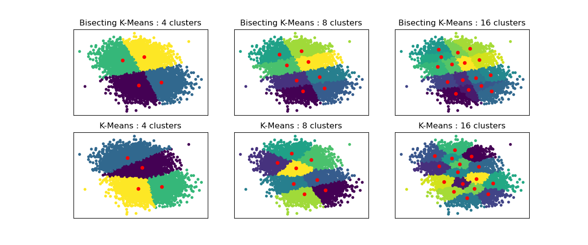
二分 K-平均和常規 K-平均效能比較#

此範例顯示常規 K-平均演算法與二分 K-平均之間的差異。

當增加 n_clusters 時，K-平均叢集有所不同，而二分 K-平均叢集則以前一個為基礎。因此，它傾向於創建具有更規則大規模結構的叢集。這種差異可以在視覺上觀察到：對於所有叢集數量，二分KMeans 都有一條將整體資料雲分為兩部分的分界線，而常規 K-平均則沒有。

Bisecting K-Means : 4 clusters, Bisecting K-Means : 8 clusters, Bisecting K-Means : 16 clusters, K-Means : 4 clusters, K-Means : 8 clusters, K-Means : 16 clusters

# Authors: The scikit-learn developers
# SPDX-License-Identifier: BSD-3-Clause

import matplotlib.pyplot as plt

from sklearn.cluster import BisectingKMeans, KMeans
from sklearn.datasets import make_blobs

print(__doc__)


# Generate sample data
n_samples = 10000
random_state = 0

X, _ = make_blobs(n_samples=n_samples, centers=2, random_state=random_state)

# Number of cluster centers for KMeans and BisectingKMeans
n_clusters_list = [4, 8, 16]

# Algorithms to compare
clustering_algorithms = {
    "Bisecting K-Means": BisectingKMeans,
    "K-Means": KMeans,
}

# Make subplots for each variant
fig, axs = plt.subplots(
    len(clustering_algorithms), len(n_clusters_list), figsize=(12, 5)
)

axs = axs.T

for i, (algorithm_name, Algorithm) in enumerate(clustering_algorithms.items()):
    for j, n_clusters in enumerate(n_clusters_list):
        algo = Algorithm(n_clusters=n_clusters, random_state=random_state, n_init=3)
        algo.fit(X)
        centers = algo.cluster_centers_

        axs[j, i].scatter(X[:, 0], X[:, 1], s=10, c=algo.labels_)
        axs[j, i].scatter(centers[:, 0], centers[:, 1], c="r", s=20)

        axs[j, i].set_title(f"{algorithm_name} : {n_clusters} clusters")


# Hide x labels and tick labels for top plots and y ticks for right plots.
for ax in axs.flat:
    ax.label_outer()
    ax.set_xticks([])
    ax.set_yticks([])

plt.show()