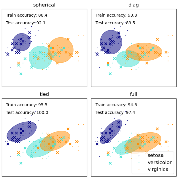
GMM 共變異數#

高斯混合模型多種共變異數類型的展示。

請參閱高斯混合模型以取得有關估計器的更多資訊。

雖然 GMM 通常用於群集，但我們可以將取得的群集與資料集的實際類別進行比較。我們使用訓練集中類別的平均值來初始化高斯分布的平均值，以使此比較有效。

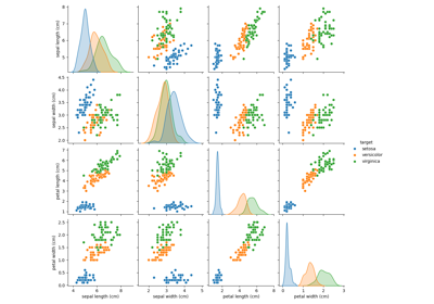
我們在鳶尾花資料集上使用各種 GMM 共變異數類型，繪製訓練和保留測試資料的預測標籤。我們比較具有球面、對角、完整和綁定共變異數矩陣的 GMM，依效能遞增順序排列。儘管通常會期望完整共變異數表現最佳，但它容易在小型資料集上過擬合，並且無法很好地推廣到保留的測試資料。

在圖中，訓練資料顯示為點，而測試資料顯示為叉號。鳶尾花資料集是四維的。此處僅顯示前兩個維度，因此某些點在其他維度中是分開的。

# Authors: The scikit-learn developers
# SPDX-License-Identifier: BSD-3-Clause

import matplotlib as mpl
import matplotlib.pyplot as plt
import numpy as np

from sklearn import datasets
from sklearn.mixture import GaussianMixture
from sklearn.model_selection import StratifiedKFold

colors = ["navy", "turquoise", "darkorange"]


def make_ellipses(gmm, ax):
    for n, color in enumerate(colors):
        if gmm.covariance_type == "full":
            covariances = gmm.covariances_[n][:2, :2]
        elif gmm.covariance_type == "tied":
            covariances = gmm.covariances_[:2, :2]
        elif gmm.covariance_type == "diag":
            covariances = np.diag(gmm.covariances_[n][:2])
        elif gmm.covariance_type == "spherical":
            covariances = np.eye(gmm.means_.shape[1]) * gmm.covariances_[n]
        v, w = np.linalg.eigh(covariances)
        u = w[0] / np.linalg.norm(w[0])
        angle = np.arctan2(u[1], u[0])
        angle = 180 * angle / np.pi  # convert to degrees
        v = 2.0 * np.sqrt(2.0) * np.sqrt(v)
        ell = mpl.patches.Ellipse(
            gmm.means_[n, :2], v[0], v[1], angle=180 + angle, color=color
        )
        ell.set_clip_box(ax.bbox)
        ell.set_alpha(0.5)
        ax.add_artist(ell)
        ax.set_aspect("equal", "datalim")


iris = datasets.load_iris()

# Break up the dataset into non-overlapping training (75%) and testing
# (25%) sets.
skf = StratifiedKFold(n_splits=4)
# Only take the first fold.
train_index, test_index = next(iter(skf.split(iris.data, iris.target)))


X_train = iris.data[train_index]
y_train = iris.target[train_index]
X_test = iris.data[test_index]
y_test = iris.target[test_index]

n_classes = len(np.unique(y_train))

# Try GMMs using different types of covariances.
estimators = {
    cov_type: GaussianMixture(
        n_components=n_classes, covariance_type=cov_type, max_iter=20, random_state=0
    )
    for cov_type in ["spherical", "diag", "tied", "full"]
}

n_estimators = len(estimators)

plt.figure(figsize=(3 * n_estimators // 2, 6))
plt.subplots_adjust(
    bottom=0.01, top=0.95, hspace=0.15, wspace=0.05, left=0.01, right=0.99
)


for index, (name, estimator) in enumerate(estimators.items()):
    # Since we have class labels for the training data, we can
    # initialize the GMM parameters in a supervised manner.
    estimator.means_init = np.array(
        [X_train[y_train == i].mean(axis=0) for i in range(n_classes)]
    )

    # Train the other parameters using the EM algorithm.
    estimator.fit(X_train)

    h = plt.subplot(2, n_estimators // 2, index + 1)
    make_ellipses(estimator, h)

    for n, color in enumerate(colors):
        data = iris.data[iris.target == n]
        plt.scatter(
            data[:, 0], data[:, 1], s=0.8, color=color, label=iris.target_names[n]
        )
    # Plot the test data with crosses
    for n, color in enumerate(colors):
        data = X_test[y_test == n]
        plt.scatter(data[:, 0], data[:, 1], marker="x", color=color)

    y_train_pred = estimator.predict(X_train)
    train_accuracy = np.mean(y_train_pred.ravel() == y_train.ravel()) * 100
    plt.text(0.05, 0.9, "Train accuracy: %.1f" % train_accuracy, transform=h.transAxes)

    y_test_pred = estimator.predict(X_test)
    test_accuracy = np.mean(y_test_pred.ravel() == y_test.ravel()) * 100
    plt.text(0.05, 0.8, "Test accuracy: %.1f" % test_accuracy, transform=h.transAxes)

    plt.xticks(())
    plt.yticks(())
    plt.title(name)

plt.legend(scatterpoints=1, loc="lower right", prop=dict(size=12))


plt.show()