具有多重共線性或相關特徵的排列重要性#

在此範例中，我們計算訓練過的 RandomForestClassifier 的特徵的 permutation_importance，使用乳癌威斯康辛 (診斷) 資料集。該模型在測試資料集上可以輕鬆獲得約 97% 的準確度。由於此資料集包含多重共線性特徵，因此排列重要性顯示沒有任何特徵是重要的，這與高測試準確度相矛盾。

我們示範了一種處理多重共線性的可能方法，該方法包括對特徵的 Spearman 秩次相關性進行層次聚類、選擇閾值，並從每個群集中保留單一特徵。

注意

另請參閱排列重要性 vs 隨機森林特徵重要性 (MDI)

# Authors: The scikit-learn developers
# SPDX-License-Identifier: BSD-3-Clause

乳癌資料上的隨機森林特徵重要性#

首先，我們定義一個函數來簡化繪圖

import matplotlib

from sklearn.inspection import permutation_importance
from sklearn.utils.fixes import parse_version


def plot_permutation_importance(clf, X, y, ax):
    result = permutation_importance(clf, X, y, n_repeats=10, random_state=42, n_jobs=2)
    perm_sorted_idx = result.importances_mean.argsort()

    # `labels` argument in boxplot is deprecated in matplotlib 3.9 and has been
    # renamed to `tick_labels`. The following code handles this, but as a
    # scikit-learn user you probably can write simpler code by using `labels=...`
    # (matplotlib < 3.9) or `tick_labels=...` (matplotlib >= 3.9).
    tick_labels_parameter_name = (
        "tick_labels"
        if parse_version(matplotlib.__version__) >= parse_version("3.9")
        else "labels"
    )
    tick_labels_dict = {tick_labels_parameter_name: X.columns[perm_sorted_idx]}
    ax.boxplot(result.importances[perm_sorted_idx].T, vert=False, **tick_labels_dict)
    ax.axvline(x=0, color="k", linestyle="--")
    return ax

然後，我們在乳癌威斯康辛 (診斷) 資料集上訓練 RandomForestClassifier，並評估其在測試集上的準確度

from sklearn.datasets import load_breast_cancer
from sklearn.ensemble import RandomForestClassifier
from sklearn.model_selection import train_test_split

X, y = load_breast_cancer(return_X_y=True, as_frame=True)
X_train, X_test, y_train, y_test = train_test_split(X, y, random_state=42)

clf = RandomForestClassifier(n_estimators=100, random_state=42)
clf.fit(X_train, y_train)
print(f"Baseline accuracy on test data: {clf.score(X_test, y_test):.2}")

Baseline accuracy on test data: 0.97

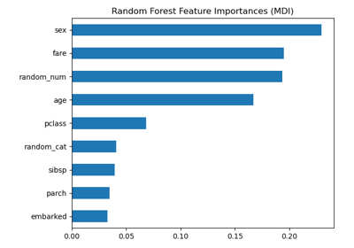
接下來，我們繪製基於樹的特徵重要性和排列重要性。排列重要性是在訓練集上計算的，以顯示模型在訓練期間依賴每個特徵的程度。

import matplotlib.pyplot as plt
import numpy as np
import pandas as pd

mdi_importances = pd.Series(clf.feature_importances_, index=X_train.columns)
tree_importance_sorted_idx = np.argsort(clf.feature_importances_)

fig, (ax1, ax2) = plt.subplots(1, 2, figsize=(12, 8))
mdi_importances.sort_values().plot.barh(ax=ax1)
ax1.set_xlabel("Gini importance")
plot_permutation_importance(clf, X_train, y_train, ax2)
ax2.set_xlabel("Decrease in accuracy score")
fig.suptitle(
    "Impurity-based vs. permutation importances on multicollinear features (train set)"
)
_ = fig.tight_layout()

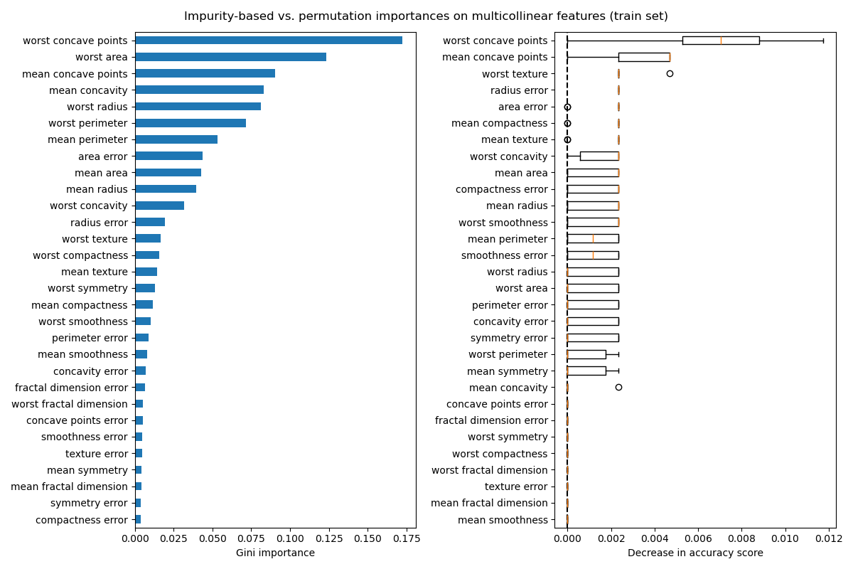
Impurity-based vs. permutation importances on multicollinear features (train set)

左側的圖顯示了模型的 Gini 重要性。由於 RandomForestClassifier 的 scikit-learn 實作在每次分割時使用 \(\sqrt{n_\text{features}}\) 個特徵的隨機子集，因此它能夠稀釋任何單一相關特徵的優勢。因此，個別特徵的重要性可能會更均勻地分佈在相關特徵之間。由於這些特徵具有較大的基數且分類器沒有過擬合，因此我們可以相對信任這些值。

右圖上的排列重要性顯示，排列一個特徵最多會使準確度下降 0.012，這表明沒有任何特徵是重要的。這與計算為基準的高測試準確度相矛盾：某些特徵一定很重要。

同樣地，在測試集上計算的準確度分數變化似乎是由於機率驅動的

fig, ax = plt.subplots(figsize=(7, 6))
plot_permutation_importance(clf, X_test, y_test, ax)
ax.set_title("Permutation Importances on multicollinear features\n(test set)")
ax.set_xlabel("Decrease in accuracy score")
_ = ax.figure.tight_layout()

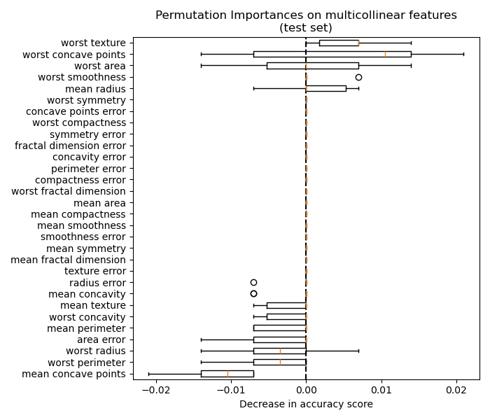
Permutation Importances on multicollinear features (test set)

儘管如此，在存在相關特徵的情況下，仍然可以計算出有意義的排列重要性，如下節所示。

處理多重共線性特徵#

當特徵共線時，排列一個特徵對模型的效能影響不大，因為它可以從相關特徵獲得相同的資訊。請注意，並非所有預測模型都是如此，這取決於它們的底層實作。

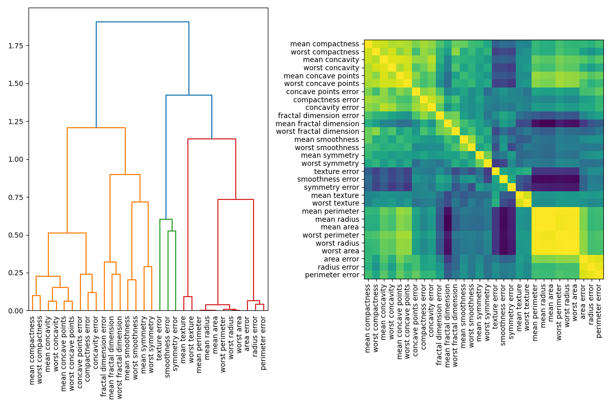
處理多重共線性特徵的一種方法是對 Spearman 秩次相關性進行層次聚類、選擇閾值，並從每個群集中保留單一特徵。首先，我們繪製相關特徵的熱圖

from scipy.cluster import hierarchy
from scipy.spatial.distance import squareform
from scipy.stats import spearmanr

fig, (ax1, ax2) = plt.subplots(1, 2, figsize=(12, 8))
corr = spearmanr(X).correlation

# Ensure the correlation matrix is symmetric
corr = (corr + corr.T) / 2
np.fill_diagonal(corr, 1)

# We convert the correlation matrix to a distance matrix before performing
# hierarchical clustering using Ward's linkage.
distance_matrix = 1 - np.abs(corr)
dist_linkage = hierarchy.ward(squareform(distance_matrix))
dendro = hierarchy.dendrogram(
    dist_linkage, labels=X.columns.to_list(), ax=ax1, leaf_rotation=90
)
dendro_idx = np.arange(0, len(dendro["ivl"]))

ax2.imshow(corr[dendro["leaves"], :][:, dendro["leaves"]])
ax2.set_xticks(dendro_idx)
ax2.set_yticks(dendro_idx)
ax2.set_xticklabels(dendro["ivl"], rotation="vertical")
ax2.set_yticklabels(dendro["ivl"])
_ = fig.tight_layout()

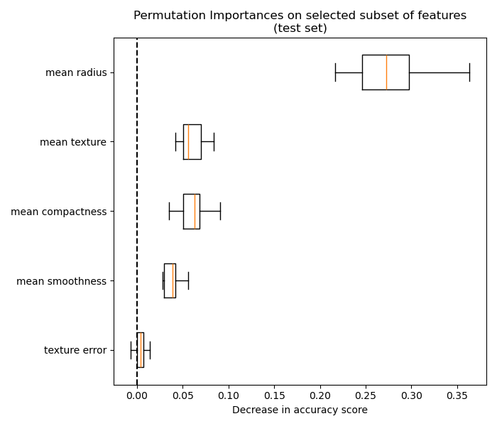
plot permutation importance multicollinear

接下來，我們透過目視檢查樹狀圖手動選擇一個閾值，將我們的特徵分組到群集中，並選擇每個群集中的一個特徵來保留，從我們的資料集中選擇這些特徵，並訓練新的隨機森林。與在完整資料集上訓練的隨機森林相比，新的隨機森林的測試準確度沒有太大變化。

from collections import defaultdict

cluster_ids = hierarchy.fcluster(dist_linkage, 1, criterion="distance")
cluster_id_to_feature_ids = defaultdict(list)
for idx, cluster_id in enumerate(cluster_ids):
    cluster_id_to_feature_ids[cluster_id].append(idx)
selected_features = [v[0] for v in cluster_id_to_feature_ids.values()]
selected_features_names = X.columns[selected_features]

X_train_sel = X_train[selected_features_names]
X_test_sel = X_test[selected_features_names]

clf_sel = RandomForestClassifier(n_estimators=100, random_state=42)
clf_sel.fit(X_train_sel, y_train)
print(
    "Baseline accuracy on test data with features removed:"
    f" {clf_sel.score(X_test_sel, y_test):.2}"
)

Baseline accuracy on test data with features removed: 0.97

我們最終可以探索所選特徵子集的排列重要性

fig, ax = plt.subplots(figsize=(7, 6))
plot_permutation_importance(clf_sel, X_test_sel, y_test, ax)
ax.set_title("Permutation Importances on selected subset of features\n(test set)")
ax.set_xlabel("Decrease in accuracy score")
ax.figure.tight_layout()
plt.show()