使用字典學習進行影像去噪#

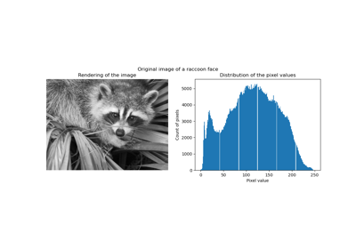
一個範例，比較首先使用線上字典學習和各種轉換方法，重建浣熊臉部影像的雜訊片段的效果。

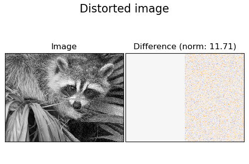
字典在影像的扭曲左半部上擬合，隨後用於重建右半部。請注意，透過擬合未失真（即無雜訊）的影像可以實現更好的效能，但這裡我們從假設它不可用的情況開始。

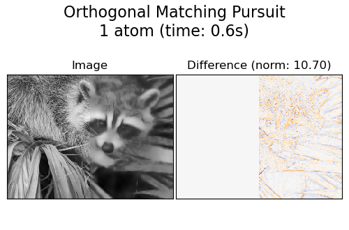
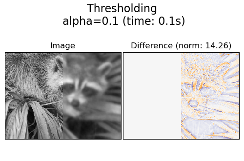
評估影像去噪結果的常見做法是查看重建影像與原始影像之間的差異。如果重建是完美的，這看起來會像高斯雜訊。

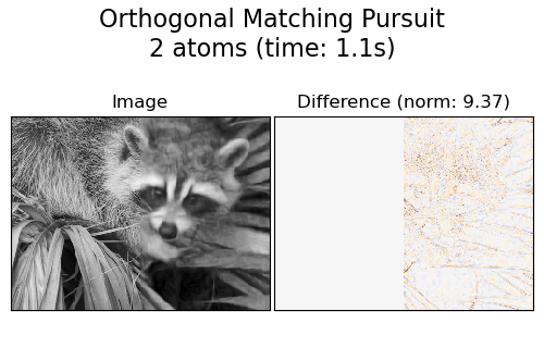
從圖中可以看出，保留兩個非零係數的正交匹配追蹤 (OMP)的結果比僅保留一個係數的結果稍微不偏（邊緣看起來不那麼突出）。此外，它在 Frobenius 範數中更接近真值。

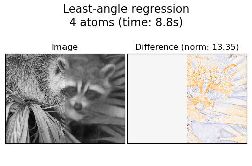
最小角迴歸的結果更強烈地偏斜：差異讓人想起原始影像的局部強度值。

閾值處理對於去噪顯然沒有用處，但這裡顯示它可以產生速度非常快的暗示性輸出，因此對於其他任務（例如物件分類）很有用，在這些任務中，效能不一定與視覺化相關。

# Authors: The scikit-learn developers
# SPDX-License-Identifier: BSD-3-Clause

產生扭曲影像#

import numpy as np

try:  # Scipy >= 1.10
    from scipy.datasets import face
except ImportError:
    from scipy.misc import face

raccoon_face = face(gray=True)

# Convert from uint8 representation with values between 0 and 255 to
# a floating point representation with values between 0 and 1.
raccoon_face = raccoon_face / 255.0

# downsample for higher speed
raccoon_face = (
    raccoon_face[::4, ::4]
    + raccoon_face[1::4, ::4]
    + raccoon_face[::4, 1::4]
    + raccoon_face[1::4, 1::4]
)
raccoon_face /= 4.0
height, width = raccoon_face.shape

# Distort the right half of the image
print("Distorting image...")
distorted = raccoon_face.copy()
distorted[:, width // 2 :] += 0.075 * np.random.randn(height, width // 2)

Distorting image...

顯示扭曲影像#

import matplotlib.pyplot as plt


def show_with_diff(image, reference, title):
    """Helper function to display denoising"""
    plt.figure(figsize=(5, 3.3))
    plt.subplot(1, 2, 1)
    plt.title("Image")
    plt.imshow(image, vmin=0, vmax=1, cmap=plt.cm.gray, interpolation="nearest")
    plt.xticks(())
    plt.yticks(())
    plt.subplot(1, 2, 2)
    difference = image - reference

    plt.title("Difference (norm: %.2f)" % np.sqrt(np.sum(difference**2)))
    plt.imshow(
        difference, vmin=-0.5, vmax=0.5, cmap=plt.cm.PuOr, interpolation="nearest"
    )
    plt.xticks(())
    plt.yticks(())
    plt.suptitle(title, size=16)
    plt.subplots_adjust(0.02, 0.02, 0.98, 0.79, 0.02, 0.2)


show_with_diff(distorted, raccoon_face, "Distorted image")

Distorted image, Image, Difference (norm: 11.71)

提取參考修補程式#

from time import time

from sklearn.feature_extraction.image import extract_patches_2d

# Extract all reference patches from the left half of the image
print("Extracting reference patches...")
t0 = time()
patch_size = (7, 7)
data = extract_patches_2d(distorted[:, : width // 2], patch_size)
data = data.reshape(data.shape[0], -1)
data -= np.mean(data, axis=0)
data /= np.std(data, axis=0)
print(f"{data.shape[0]} patches extracted in %.2fs." % (time() - t0))

Extracting reference patches...
22692 patches extracted in 0.01s.

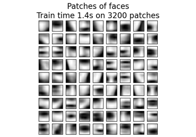
從參考修補程式學習字典#

from sklearn.decomposition import MiniBatchDictionaryLearning

print("Learning the dictionary...")
t0 = time()
dico = MiniBatchDictionaryLearning(
    # increase to 300 for higher quality results at the cost of slower
    # training times.
    n_components=50,
    batch_size=200,
    alpha=1.0,
    max_iter=10,
)
V = dico.fit(data).components_
dt = time() - t0
print(f"{dico.n_iter_} iterations / {dico.n_steps_} steps in {dt:.2f}.")

plt.figure(figsize=(4.2, 4))
for i, comp in enumerate(V[:100]):
    plt.subplot(10, 10, i + 1)
    plt.imshow(comp.reshape(patch_size), cmap=plt.cm.gray_r, interpolation="nearest")
    plt.xticks(())
    plt.yticks(())
plt.suptitle(
    "Dictionary learned from face patches\n"
    + "Train time %.1fs on %d patches" % (dt, len(data)),
    fontsize=16,
)
plt.subplots_adjust(0.08, 0.02, 0.92, 0.85, 0.08, 0.23)

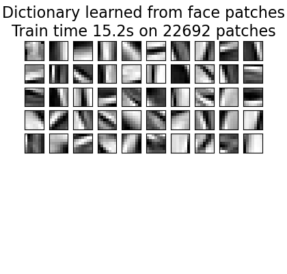
Dictionary learned from face patches Train time 15.2s on 22692 patches

Learning the dictionary...
2.0 iterations / 125 steps in 15.16.

提取雜訊修補程式並使用字典重建它們#

from sklearn.feature_extraction.image import reconstruct_from_patches_2d

print("Extracting noisy patches... ")
t0 = time()
data = extract_patches_2d(distorted[:, width // 2 :], patch_size)
data = data.reshape(data.shape[0], -1)
intercept = np.mean(data, axis=0)
data -= intercept
print("done in %.2fs." % (time() - t0))

transform_algorithms = [
    ("Orthogonal Matching Pursuit\n1 atom", "omp", {"transform_n_nonzero_coefs": 1}),
    ("Orthogonal Matching Pursuit\n2 atoms", "omp", {"transform_n_nonzero_coefs": 2}),
    ("Least-angle regression\n4 atoms", "lars", {"transform_n_nonzero_coefs": 4}),
    ("Thresholding\n alpha=0.1", "threshold", {"transform_alpha": 0.1}),
]

reconstructions = {}
for title, transform_algorithm, kwargs in transform_algorithms:
    print(title + "...")
    reconstructions[title] = raccoon_face.copy()
    t0 = time()
    dico.set_params(transform_algorithm=transform_algorithm, **kwargs)
    code = dico.transform(data)
    patches = np.dot(code, V)

    patches += intercept
    patches = patches.reshape(len(data), *patch_size)
    if transform_algorithm == "threshold":
        patches -= patches.min()
        patches /= patches.max()
    reconstructions[title][:, width // 2 :] = reconstruct_from_patches_2d(
        patches, (height, width // 2)
    )
    dt = time() - t0
    print("done in %.2fs." % dt)
    show_with_diff(reconstructions[title], raccoon_face, title + " (time: %.1fs)" % dt)

plt.show()

Extracting noisy patches...
done in 0.00s.
Orthogonal Matching Pursuit
1 atom...
done in 0.59s.
Orthogonal Matching Pursuit
2 atoms...
done in 1.14s.
Least-angle regression
4 atoms...
done in 8.76s.
Thresholding
 alpha=0.1...
done in 0.09s.

腳本的總執行時間： (0 分鐘 27.032 秒)