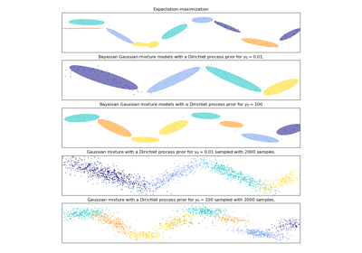
變異貝氏高斯混合模型分析的濃度先驗類型#

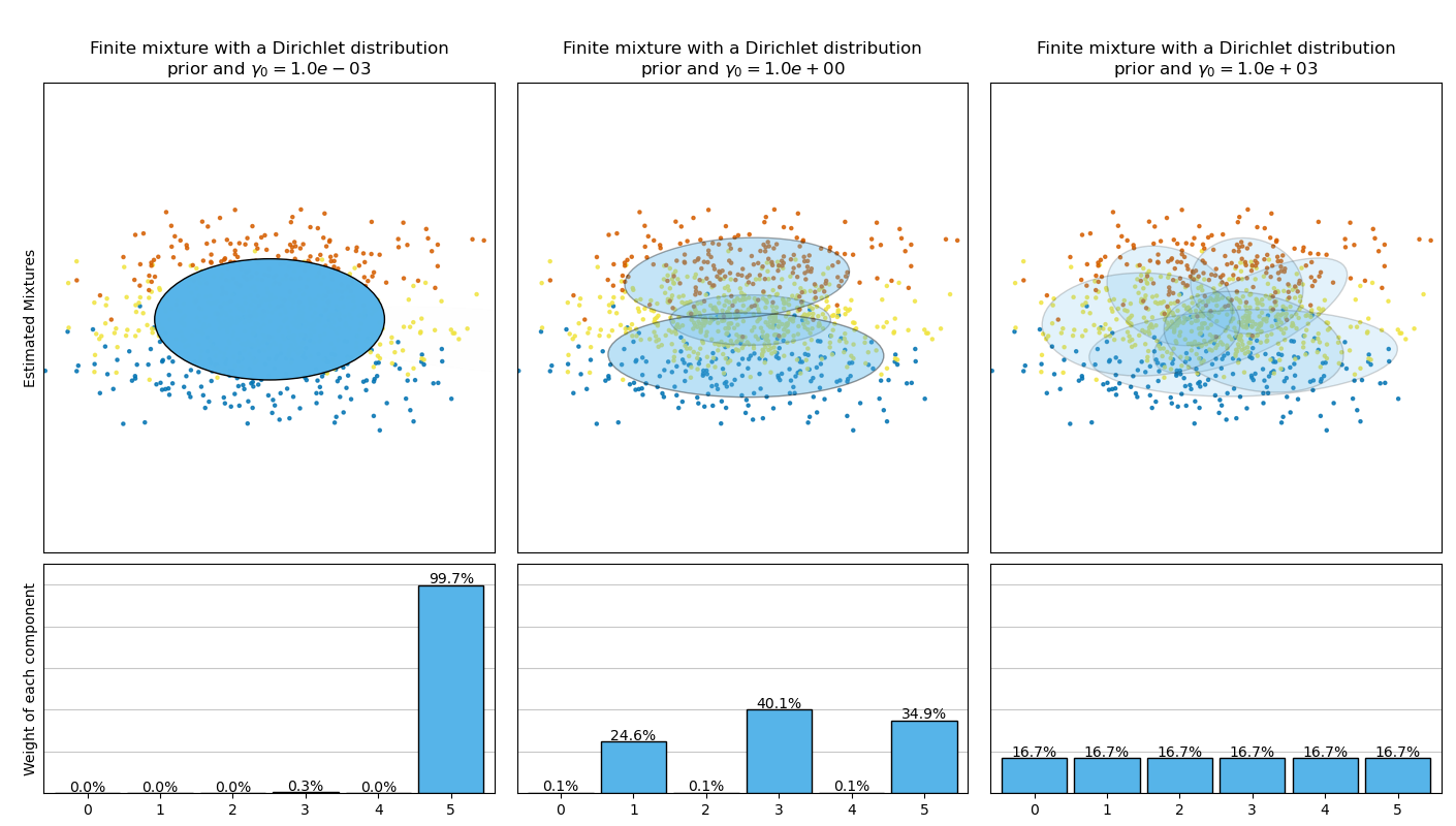
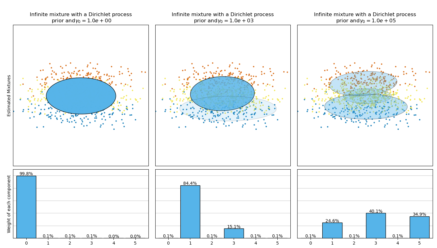
此範例繪製從玩具資料集（三個高斯分佈的混合）取得的橢圓體，這些橢圓體由具有狄利克雷分佈先驗 (weight_concentration_prior_type='dirichlet_distribution') 和狄利克雷過程先驗 (weight_concentration_prior_type='dirichlet_process') 的 BayesianGaussianMixture 類別模型擬合。在每個圖中，我們繪製三個不同權重濃度先驗值結果。

BayesianGaussianMixture 類別可以自動調整其混合成分的數量。參數 weight_concentration_prior 與具有非零權重的成分的結果數量有直接關係。為濃度先驗指定較低的值將使模型將大部分權重放在少數成分上，並將剩餘成分權重設置得非常接近零。濃度先驗的較高值將允許較多的成分在混合中處於活動狀態。

狄利克雷過程先驗允許定義無限數量的成分，並自動選擇正確的成分數量：它僅在必要時才啟動一個成分。

相反，具有狄利克雷分佈先驗的經典有限混合模型將偏向於權重更均勻的成分，因此傾向於將自然叢集分成不必要的子成分。

$Finite mixture with a Dirichlet distribution prior and $\gamma_0=$$1.0e-03$, Finite mixture with a Dirichlet distribution prior and $\gamma_0=$$1.0e+00$, Finite mixture with a Dirichlet distribution prior and $\gamma_0=$$1.0e+03$$
$Infinite mixture with a Dirichlet process prior and$\gamma_0=$$1.0e+00$, Infinite mixture with a Dirichlet process prior and$\gamma_0=$$1.0e+03$, Infinite mixture with a Dirichlet process prior and$\gamma_0=$$1.0e+05$$

# Authors: The scikit-learn developers
# SPDX-License-Identifier: BSD-3-Clause

import matplotlib as mpl
import matplotlib.gridspec as gridspec
import matplotlib.pyplot as plt
import numpy as np

from sklearn.mixture import BayesianGaussianMixture


def plot_ellipses(ax, weights, means, covars):
    for n in range(means.shape[0]):
        eig_vals, eig_vecs = np.linalg.eigh(covars[n])
        unit_eig_vec = eig_vecs[0] / np.linalg.norm(eig_vecs[0])
        angle = np.arctan2(unit_eig_vec[1], unit_eig_vec[0])
        # Ellipse needs degrees
        angle = 180 * angle / np.pi
        # eigenvector normalization
        eig_vals = 2 * np.sqrt(2) * np.sqrt(eig_vals)
        ell = mpl.patches.Ellipse(
            means[n], eig_vals[0], eig_vals[1], angle=180 + angle, edgecolor="black"
        )
        ell.set_clip_box(ax.bbox)
        ell.set_alpha(weights[n])
        ell.set_facecolor("#56B4E9")
        ax.add_artist(ell)


def plot_results(ax1, ax2, estimator, X, y, title, plot_title=False):
    ax1.set_title(title)
    ax1.scatter(X[:, 0], X[:, 1], s=5, marker="o", color=colors[y], alpha=0.8)
    ax1.set_xlim(-2.0, 2.0)
    ax1.set_ylim(-3.0, 3.0)
    ax1.set_xticks(())
    ax1.set_yticks(())
    plot_ellipses(ax1, estimator.weights_, estimator.means_, estimator.covariances_)

    ax2.get_xaxis().set_tick_params(direction="out")
    ax2.yaxis.grid(True, alpha=0.7)
    for k, w in enumerate(estimator.weights_):
        ax2.bar(
            k,
            w,
            width=0.9,
            color="#56B4E9",
            zorder=3,
            align="center",
            edgecolor="black",
        )
        ax2.text(k, w + 0.007, "%.1f%%" % (w * 100.0), horizontalalignment="center")
    ax2.set_xlim(-0.6, 2 * n_components - 0.4)
    ax2.set_ylim(0.0, 1.1)
    ax2.tick_params(axis="y", which="both", left=False, right=False, labelleft=False)
    ax2.tick_params(axis="x", which="both", top=False)

    if plot_title:
        ax1.set_ylabel("Estimated Mixtures")
        ax2.set_ylabel("Weight of each component")


# Parameters of the dataset
random_state, n_components, n_features = 2, 3, 2
colors = np.array(["#0072B2", "#F0E442", "#D55E00"])

covars = np.array(
    [[[0.7, 0.0], [0.0, 0.1]], [[0.5, 0.0], [0.0, 0.1]], [[0.5, 0.0], [0.0, 0.1]]]
)
samples = np.array([200, 500, 200])
means = np.array([[0.0, -0.70], [0.0, 0.0], [0.0, 0.70]])

# mean_precision_prior= 0.8 to minimize the influence of the prior
estimators = [
    (
        "Finite mixture with a Dirichlet distribution\nprior and " r"$\gamma_0=$",
        BayesianGaussianMixture(
            weight_concentration_prior_type="dirichlet_distribution",
            n_components=2 * n_components,
            reg_covar=0,
            init_params="random",
            max_iter=1500,
            mean_precision_prior=0.8,
            random_state=random_state,
        ),
        [0.001, 1, 1000],
    ),
    (
        "Infinite mixture with a Dirichlet process\n prior and" r"$\gamma_0=$",
        BayesianGaussianMixture(
            weight_concentration_prior_type="dirichlet_process",
            n_components=2 * n_components,
            reg_covar=0,
            init_params="random",
            max_iter=1500,
            mean_precision_prior=0.8,
            random_state=random_state,
        ),
        [1, 1000, 100000],
    ),
]

# Generate data
rng = np.random.RandomState(random_state)
X = np.vstack(
    [
        rng.multivariate_normal(means[j], covars[j], samples[j])
        for j in range(n_components)
    ]
)
y = np.concatenate([np.full(samples[j], j, dtype=int) for j in range(n_components)])

# Plot results in two different figures
for title, estimator, concentrations_prior in estimators:
    plt.figure(figsize=(4.7 * 3, 8))
    plt.subplots_adjust(
        bottom=0.04, top=0.90, hspace=0.05, wspace=0.05, left=0.03, right=0.99
    )

    gs = gridspec.GridSpec(3, len(concentrations_prior))
    for k, concentration in enumerate(concentrations_prior):
        estimator.weight_concentration_prior = concentration
        estimator.fit(X)
        plot_results(
            plt.subplot(gs[0:2, k]),
            plt.subplot(gs[2, k]),
            estimator,
            X,
            y,
            r"%s$%.1e$" % (title, concentration),
            plot_title=k == 0,
        )

plt.show()