注意
前往末尾以下載完整的範例程式碼。 或透過 JupyterLite 或 Binder 在您的瀏覽器中執行此範例
FeatureHasher 和 DictVectorizer 比較#
在此範例中,我們說明文字向量化,也就是將非數值輸入數據(例如字典或文字文件)表示為實數向量的過程。
我們首先比較 FeatureHasher 和 DictVectorizer,方法是使用這兩種方法將使用自訂 Python 函式預處理(分詞)的文字文件向量化。
稍後,我們將介紹並分析特定於文字的向量化器 HashingVectorizer、CountVectorizer 和 TfidfVectorizer,它們可以在單個類別中處理分詞和組裝特徵矩陣。
此範例的目的是示範文字向量化 API 的用法,並比較其處理時間。 請參閱範例腳本 使用稀疏特徵對文本文件進行分類 和 使用 k-means 聚類文本文件 以了解實際的文本文件學習。
# Authors: The scikit-learn developers
# SPDX-License-Identifier: BSD-3-Clause
載入數據#
我們從 20 個新聞群組文本數據集 載入數據,該數據集包含約 18000 個關於 20 個主題的新聞群組文章,分為兩個子集:一個用於訓練,另一個用於測試。 為了簡單起見並降低計算成本,我們選擇 7 個主題的子集,並且僅使用訓練集。
from sklearn.datasets import fetch_20newsgroups

categories = [
    "alt.atheism",
    "comp.graphics",
    "comp.sys.ibm.pc.hardware",
    "misc.forsale",
    "rec.autos",
    "sci.space",
    "talk.religion.misc",
]

print("Loading 20 newsgroups training data")
raw_data, _ = fetch_20newsgroups(subset="train", categories=categories, return_X_y=True)
data_size_mb = sum(len(s.encode("utf-8")) for s in raw_data) / 1e6
print(f"{len(raw_data)} documents - {data_size_mb:.3f}MB")
Loading 20 newsgroups training data
3803 documents - 6.245MB
定義預處理函式#
符記可能是單字、單字的一部分或字串中空格或符號之間包含的任何內容。 在這裡,我們定義一個使用簡單的正規表示式 (regex) 擷取符記的函式,該函式會比對 Unicode 單字字元。 這包括任何語言中可以成為單字一部分的大多數字元,以及數字和底線
import re


def tokenize(doc):
    """Extract tokens from doc.

    This uses a simple regex that matches word characters to break strings
    into tokens. For a more principled approach, see CountVectorizer or
    TfidfVectorizer.
    """
    return (tok.lower() for tok in re.findall(r"\w+", doc))


list(tokenize("This is a simple example, isn't it?"))
['this', 'is', 'a', 'simple', 'example', 'isn', 't', 'it']
我們定義一個額外的函式,用於計算給定文件中每個符記的出現次數(頻率)。 它會傳回一個頻率字典,供向量化器使用。
from collections import defaultdict


def token_freqs(doc):
    """Extract a dict mapping tokens from doc to their occurrences."""

    freq = defaultdict(int)
    for tok in tokenize(doc):
        freq[tok] += 1
    return freq


token_freqs("That is one example, but this is another one")
defaultdict(<class 'int'>, {'that': 1, 'is': 2, 'one': 2, 'example': 1, 'but': 1, 'this': 1, 'another': 1})
請特別注意,重複的符記 "is" 例如計算兩次。
將文本文件分解為單字符記,可能會遺失句子中單字之間的順序資訊,這通常稱為 詞袋表示。
DictVectorizer#
首先,我們對 DictVectorizer 進行基準測試,然後將其與 FeatureHasher 進行比較,因為它們都接收字典作為輸入。
from time import time

from sklearn.feature_extraction import DictVectorizer

dict_count_vectorizers = defaultdict(list)

t0 = time()
vectorizer = DictVectorizer()
vectorizer.fit_transform(token_freqs(d) for d in raw_data)
duration = time() - t0
dict_count_vectorizers["vectorizer"].append(
    vectorizer.__class__.__name__ + "\non freq dicts"
)
dict_count_vectorizers["speed"].append(data_size_mb / duration)
print(f"done in {duration:.3f} s at {data_size_mb / duration:.1f} MB/s")
print(f"Found {len(vectorizer.get_feature_names_out())} unique terms")
done in 1.162 s at 5.4 MB/s
Found 47928 unique terms
從文字符記到欄索引的實際對應明確儲存在 .vocabulary_ 屬性中,這是一個潛在非常大的 Python 字典
type(vectorizer.vocabulary_)
len(vectorizer.vocabulary_)
47928
vectorizer.vocabulary_["example"]
19145
FeatureHasher#
字典會佔用大量的儲存空間,並且隨著訓練集的增長而增大。 特徵雜湊不是隨著字典一起增長向量,而是透過將雜湊函式 h 套用至特徵(例如,符記),然後直接使用雜湊值作為特徵索引,並在這些索引中更新產生的向量,來建構預先定義長度的向量。 當特徵空間不夠大時,雜湊函式會傾向於將不同的值對應到相同的雜湊碼(雜湊碰撞)。 因此,無法判斷哪個物件產生了任何特定的雜湊碼。
由於以上原因,無法從特徵矩陣復原原始符記,而估計原始字典中唯一術語數量的最佳方法是計算編碼特徵矩陣中活動欄的數量。 為此,我們定義以下函式
import numpy as np


def n_nonzero_columns(X):
    """Number of columns with at least one non-zero value in a CSR matrix.

    This is useful to count the number of features columns that are effectively
    active when using the FeatureHasher.
    """
    return len(np.unique(X.nonzero()[1]))
FeatureHasher 的預設特徵數為 2**20。 在這裡,我們設定 n_features = 2**18 以說明雜湊碰撞。
頻率字典上的 FeatureHasher
from sklearn.feature_extraction import FeatureHasher

t0 = time()
hasher = FeatureHasher(n_features=2**18)
X = hasher.transform(token_freqs(d) for d in raw_data)
duration = time() - t0
dict_count_vectorizers["vectorizer"].append(
    hasher.__class__.__name__ + "\non freq dicts"
)
dict_count_vectorizers["speed"].append(data_size_mb / duration)
print(f"done in {duration:.3f} s at {data_size_mb / duration:.1f} MB/s")
print(f"Found {n_nonzero_columns(X)} unique tokens")
done in 0.574 s at 10.9 MB/s
Found 43873 unique tokens
使用 FeatureHasher 時的唯一符記數少於使用 DictVectorizer 取得的符記數。 這是由於雜湊碰撞所致。
可以透過增加特徵空間來減少碰撞次數。 請注意,當設定大量特徵時,向量化器的速度不會顯著改變,儘管它會導致更大的係數維度,然後需要更多的記憶體來儲存它們,即使它們中的大多數處於非活動狀態。
t0 = time()
hasher = FeatureHasher(n_features=2**22)
X = hasher.transform(token_freqs(d) for d in raw_data)
duration = time() - t0

print(f"done in {duration:.3f} s at {data_size_mb / duration:.1f} MB/s")
print(f"Found {n_nonzero_columns(X)} unique tokens")
done in 0.575 s at 10.9 MB/s
Found 47668 unique tokens
我們確認唯一符記的數量會更接近 DictVectorizer 找到的唯一術語數量。
原始符記上的 FeatureHasher
或者,您可以在 FeatureHasher 中設定 input_type="string",以直接將自訂 tokenize 函式輸出的字串向量化。 這相當於傳遞一個字典,其中每個特徵名稱的隱含頻率為 1。
t0 = time()
hasher = FeatureHasher(n_features=2**18, input_type="string")
X = hasher.transform(tokenize(d) for d in raw_data)
duration = time() - t0
dict_count_vectorizers["vectorizer"].append(
    hasher.__class__.__name__ + "\non raw tokens"
)
dict_count_vectorizers["speed"].append(data_size_mb / duration)
print(f"done in {duration:.3f} s at {data_size_mb / duration:.1f} MB/s")
print(f"Found {n_nonzero_columns(X)} unique tokens")
done in 0.543 s at 11.5 MB/s
Found 43873 unique tokens
現在,我們繪製上述向量化方法的速度。
import matplotlib.pyplot as plt

fig, ax = plt.subplots(figsize=(12, 6))

y_pos = np.arange(len(dict_count_vectorizers["vectorizer"]))
ax.barh(y_pos, dict_count_vectorizers["speed"], align="center")
ax.set_yticks(y_pos)
ax.set_yticklabels(dict_count_vectorizers["vectorizer"])
ax.invert_yaxis()
_ = ax.set_xlabel("speed (MB/s)")
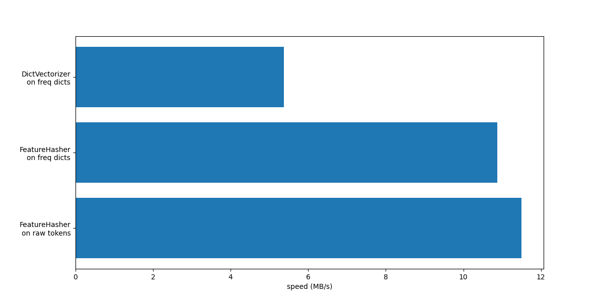
在這兩種情況下,FeatureHasher 的速度大約是 DictVectorizer 的兩倍。 這在處理大量數據時很方便,缺點是會失去轉換的可逆性,這反過來使模型的解釋變得更加複雜。
使用 input_type="string" 的 FeatureHeasher 比處理詞頻字典的版本稍微快一些,因為它不會計算重複的詞彙:即使詞彙重複出現,每個詞彙也只會被隱含地計算一次。根據下游的機器學習任務,這可能是一個限制,也可能不是。
與專用文字向量化器的比較#
CountVectorizer 接受原始數據,因為它內部實作了分詞和詞彙計數。它類似於 DictVectorizer,當與自定義函數 token_freqs 一起使用時,如前一節所述。不同之處在於 CountVectorizer 更加靈活。特別是,它透過 token_pattern 參數接受各種正則表達式模式。
from sklearn.feature_extraction.text import CountVectorizer

t0 = time()
vectorizer = CountVectorizer()
vectorizer.fit_transform(raw_data)
duration = time() - t0
dict_count_vectorizers["vectorizer"].append(vectorizer.__class__.__name__)
dict_count_vectorizers["speed"].append(data_size_mb / duration)
print(f"done in {duration:.3f} s at {data_size_mb / duration:.1f} MB/s")
print(f"Found {len(vectorizer.get_feature_names_out())} unique terms")
done in 0.714 s at 8.7 MB/s
Found 47885 unique terms
我們看到,使用 CountVectorizer 的實作大約比使用 DictVectorizer 以及我們為映射詞彙所定義的簡單函數快兩倍。原因在於 CountVectorizer 透過為整個訓練集重複使用編譯過的正則表達式進行優化,而不是像我們簡單的分詞函數那樣為每個文件創建一個正則表達式。
現在,我們使用 HashingVectorizer 進行類似的實驗,它相當於結合了 FeatureHasher 類別所實作的「雜湊技巧」和 CountVectorizer 的文字預處理和分詞。
from sklearn.feature_extraction.text import HashingVectorizer

t0 = time()
vectorizer = HashingVectorizer(n_features=2**18)
vectorizer.fit_transform(raw_data)
duration = time() - t0
dict_count_vectorizers["vectorizer"].append(vectorizer.__class__.__name__)
dict_count_vectorizers["speed"].append(data_size_mb / duration)
print(f"done in {duration:.3f} s at {data_size_mb / duration:.1f} MB/s")
done in 0.511 s at 12.2 MB/s
我們可以觀察到,這是目前最快的文字分詞策略,假設下游的機器學習任務可以容忍一些碰撞。
TfidfVectorizer#
在大型文字語料庫中,有些詞彙出現的頻率較高(例如,英文中的 “the”、“a”、“is”),並且沒有攜帶關於文件實際內容的有意義資訊。如果我們直接將詞彙計數數據輸入分類器,這些非常常見的詞彙將會掩蓋較罕見但資訊量更大的詞彙的頻率。為了將計數特徵重新加權為適合分類器使用的浮點數值,通常會使用由 TfidfTransformer 實作的 tf-idf 轉換。TF 代表「詞彙頻率 (term-frequency)」,而 “tf-idf” 則表示詞彙頻率乘以逆向文件頻率 (inverse document-frequency)。
我們現在對 TfidfVectorizer 進行基準測試,它相當於結合了 CountVectorizer 的分詞和詞彙計數,以及來自 TfidfTransformer 的正規化和加權。
from sklearn.feature_extraction.text import TfidfVectorizer

t0 = time()
vectorizer = TfidfVectorizer()
vectorizer.fit_transform(raw_data)
duration = time() - t0
dict_count_vectorizers["vectorizer"].append(vectorizer.__class__.__name__)
dict_count_vectorizers["speed"].append(data_size_mb / duration)
print(f"done in {duration:.3f} s at {data_size_mb / duration:.1f} MB/s")
print(f"Found {len(vectorizer.get_feature_names_out())} unique terms")
done in 0.717 s at 8.7 MB/s
Found 47885 unique terms
總結#
讓我們透過在單一圖表中總結所有記錄的處理速度來結束本筆記本。
fig, ax = plt.subplots(figsize=(12, 6))

y_pos = np.arange(len(dict_count_vectorizers["vectorizer"]))
ax.barh(y_pos, dict_count_vectorizers["speed"], align="center")
ax.set_yticks(y_pos)
ax.set_yticklabels(dict_count_vectorizers["vectorizer"])
ax.invert_yaxis()
_ = ax.set_xlabel("speed (MB/s)")
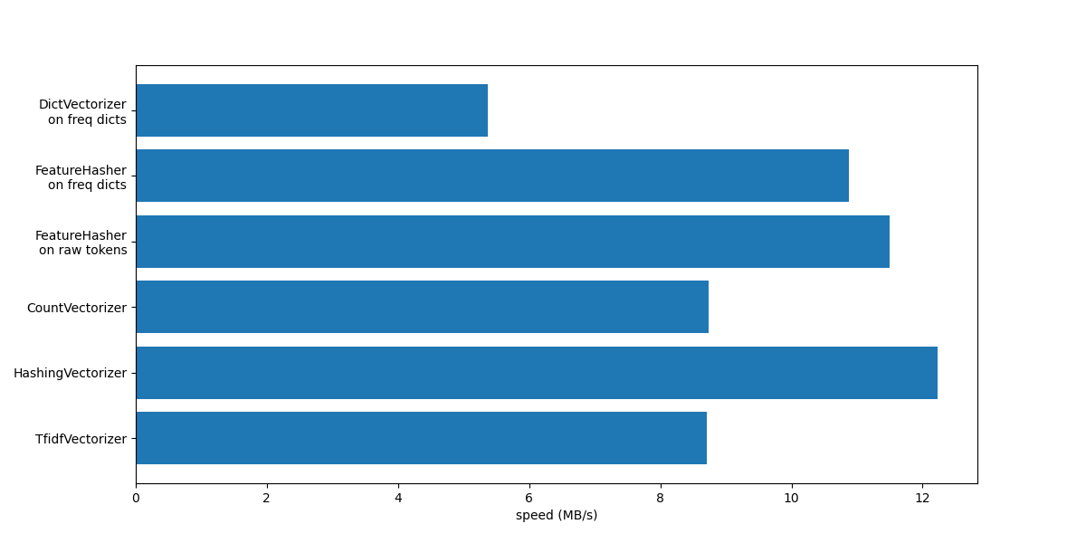
從圖表中注意到,由於 TfidfTransformer 引起的額外操作,TfidfVectorizer 比 CountVectorizer 稍微慢一些。
另請注意,透過設定特徵數量 n_features = 2**18,HashingVectorizer 的效能優於 CountVectorizer,但代價是由於雜湊碰撞導致轉換不可逆。
我們強調,CountVectorizer 和 HashingVectorizer 的效能優於它們在手動分詞文件上的對應物 DictVectorizer 和 FeatureHasher,因為前者向量化器的內部分詞步驟會編譯一次正則表達式,然後將其重複用於所有文件。
腳本總執行時間: (0 分鐘 5.279 秒)
相關範例