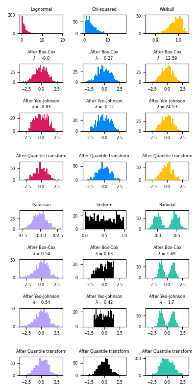
將資料對應到常態分佈

此範例示範如何使用 Box-Cox 和 Yeo-Johnson 轉換，透過 PowerTransformer 將來自各種分佈的資料對應到常態分佈。

當需要同方差性和常態性時，冪轉換在建模問題中很有用。以下是 Box-Cox 和 Yeo-Johnwon 應用於六種不同機率分佈的範例：對數常態、卡方、韋伯、高斯、均勻和雙峰。

請注意，當轉換應用於某些資料集時，它們會成功地將資料對應到常態分佈，但對其他資料集無效。這突顯了在轉換前後視覺化資料的重要性。

另請注意，即使 Box-Cox 在對數常態和卡方分佈方面似乎比 Yeo-Johnson 表現更好，但請記住 Box-Cox 不支援具有負值的輸入。

為了比較，我們還添加了來自 QuantileTransformer 的輸出。它可以將任何任意分佈強制轉換為高斯分佈，前提是有足夠的訓練樣本（數千個）。由於它是一種非參數方法，因此比參數方法（Box-Cox 和 Yeo-Johnson）更難解釋。

在「小型」資料集（少於數百個點）上，分位數轉換器容易過擬合。建議使用冪轉換。

# Authors: The scikit-learn developers
# SPDX-License-Identifier: BSD-3-Clause

import matplotlib.pyplot as plt
import numpy as np

from sklearn.model_selection import train_test_split
from sklearn.preprocessing import PowerTransformer, QuantileTransformer

N_SAMPLES = 1000
FONT_SIZE = 6
BINS = 30


rng = np.random.RandomState(304)
bc = PowerTransformer(method="box-cox")
yj = PowerTransformer(method="yeo-johnson")
# n_quantiles is set to the training set size rather than the default value
# to avoid a warning being raised by this example
qt = QuantileTransformer(
    n_quantiles=500, output_distribution="normal", random_state=rng
)
size = (N_SAMPLES, 1)


# lognormal distribution
X_lognormal = rng.lognormal(size=size)

# chi-squared distribution
df = 3
X_chisq = rng.chisquare(df=df, size=size)

# weibull distribution
a = 50
X_weibull = rng.weibull(a=a, size=size)

# gaussian distribution
loc = 100
X_gaussian = rng.normal(loc=loc, size=size)

# uniform distribution
X_uniform = rng.uniform(low=0, high=1, size=size)

# bimodal distribution
loc_a, loc_b = 100, 105
X_a, X_b = rng.normal(loc=loc_a, size=size), rng.normal(loc=loc_b, size=size)
X_bimodal = np.concatenate([X_a, X_b], axis=0)


# create plots
distributions = [
    ("Lognormal", X_lognormal),
    ("Chi-squared", X_chisq),
    ("Weibull", X_weibull),
    ("Gaussian", X_gaussian),
    ("Uniform", X_uniform),
    ("Bimodal", X_bimodal),
]

colors = ["#D81B60", "#0188FF", "#FFC107", "#B7A2FF", "#000000", "#2EC5AC"]

fig, axes = plt.subplots(nrows=8, ncols=3, figsize=plt.figaspect(2))
axes = axes.flatten()
axes_idxs = [
    (0, 3, 6, 9),
    (1, 4, 7, 10),
    (2, 5, 8, 11),
    (12, 15, 18, 21),
    (13, 16, 19, 22),
    (14, 17, 20, 23),
]
axes_list = [(axes[i], axes[j], axes[k], axes[l]) for (i, j, k, l) in axes_idxs]


for distribution, color, axes in zip(distributions, colors, axes_list):
    name, X = distribution
    X_train, X_test = train_test_split(X, test_size=0.5)

    # perform power transforms and quantile transform
    X_trans_bc = bc.fit(X_train).transform(X_test)
    lmbda_bc = round(bc.lambdas_[0], 2)
    X_trans_yj = yj.fit(X_train).transform(X_test)
    lmbda_yj = round(yj.lambdas_[0], 2)
    X_trans_qt = qt.fit(X_train).transform(X_test)

    ax_original, ax_bc, ax_yj, ax_qt = axes

    ax_original.hist(X_train, color=color, bins=BINS)
    ax_original.set_title(name, fontsize=FONT_SIZE)
    ax_original.tick_params(axis="both", which="major", labelsize=FONT_SIZE)

    for ax, X_trans, meth_name, lmbda in zip(
        (ax_bc, ax_yj, ax_qt),
        (X_trans_bc, X_trans_yj, X_trans_qt),
        ("Box-Cox", "Yeo-Johnson", "Quantile transform"),
        (lmbda_bc, lmbda_yj, None),
    ):
        ax.hist(X_trans, color=color, bins=BINS)
        title = "After {}".format(meth_name)
        if lmbda is not None:
            title += "\n$\\lambda$ = {}".format(lmbda)
        ax.set_title(title, fontsize=FONT_SIZE)
        ax.tick_params(axis="both", which="major", labelsize=FONT_SIZE)
        ax.set_xlim([-3.5, 3.5])


plt.tight_layout()
plt.show()

相關範例

比較不同縮放器對含離群值資料的影響

比較不同縮放器對含離群值資料的影響

梯度提升中的提前停止

梯度提升中的提前停止

繪製分類機率

繪製分類機率

縮放 SVC 的正規化參數

縮放 SVC 的正規化參數