階層式分群：結構化 vs 非結構化 Ward#

範例建立瑞士捲資料集並在其位置上執行階層式分群。

如需更多資訊，請參閱階層式分群。

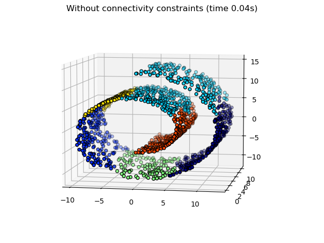
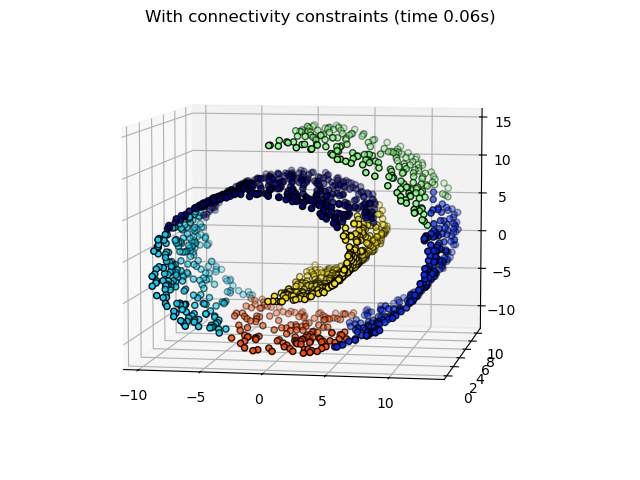
第一步，在沒有結構連通性限制的情況下執行階層式分群，並且僅基於距離，而在第二步中，分群被限制為 k-Nearest Neighbors 圖：這是一個具有結構先驗的階層式分群。

一些在沒有連通性限制的情況下學習到的分群不尊重瑞士捲的結構，並且延伸到多個流形褶皺。相反地，當反對連通性限制時，分群會形成瑞士捲的良好分割。

# Authors: The scikit-learn developers
# SPDX-License-Identifier: BSD-3-Clause

import time as time

# The following import is required
# for 3D projection to work with matplotlib < 3.2
import mpl_toolkits.mplot3d  # noqa: F401
import numpy as np

產生資料#

我們首先產生瑞士捲資料集。

from sklearn.datasets import make_swiss_roll

n_samples = 1500
noise = 0.05
X, _ = make_swiss_roll(n_samples, noise=noise)
# Make it thinner
X[:, 1] *= 0.5

計算分群#

我們執行 AgglomerativeClustering，它屬於沒有任何連通性限制的階層式分群。

from sklearn.cluster import AgglomerativeClustering

print("Compute unstructured hierarchical clustering...")
st = time.time()
ward = AgglomerativeClustering(n_clusters=6, linkage="ward").fit(X)
elapsed_time = time.time() - st
label = ward.labels_
print(f"Elapsed time: {elapsed_time:.2f}s")
print(f"Number of points: {label.size}")

Compute unstructured hierarchical clustering...
Elapsed time: 0.04s
Number of points: 1500

繪製結果#

繪製非結構化的階層式分群。

import matplotlib.pyplot as plt

fig1 = plt.figure()
ax1 = fig1.add_subplot(111, projection="3d", elev=7, azim=-80)
ax1.set_position([0, 0, 0.95, 1])
for l in np.unique(label):
    ax1.scatter(
        X[label == l, 0],
        X[label == l, 1],
        X[label == l, 2],
        color=plt.cm.jet(float(l) / np.max(label + 1)),
        s=20,
        edgecolor="k",
    )
_ = fig1.suptitle(f"Without connectivity constraints (time {elapsed_time:.2f}s)")

Without connectivity constraints (time 0.04s)

我們正在定義具有 10 個鄰居的 k-Nearest Neighbors#

from sklearn.neighbors import kneighbors_graph

connectivity = kneighbors_graph(X, n_neighbors=10, include_self=False)

計算分群#

我們再次執行具有連通性限制的 AgglomerativeClustering。

print("Compute structured hierarchical clustering...")
st = time.time()
ward = AgglomerativeClustering(
    n_clusters=6, connectivity=connectivity, linkage="ward"
).fit(X)
elapsed_time = time.time() - st
label = ward.labels_
print(f"Elapsed time: {elapsed_time:.2f}s")
print(f"Number of points: {label.size}")

Compute structured hierarchical clustering...
Elapsed time: 0.06s
Number of points: 1500

繪製結果#

繪製結構化的階層式分群。

fig2 = plt.figure()
ax2 = fig2.add_subplot(121, projection="3d", elev=7, azim=-80)
ax2.set_position([0, 0, 0.95, 1])
for l in np.unique(label):
    ax2.scatter(
        X[label == l, 0],
        X[label == l, 1],
        X[label == l, 2],
        color=plt.cm.jet(float(l) / np.max(label + 1)),
        s=20,
        edgecolor="k",
    )
fig2.suptitle(f"With connectivity constraints (time {elapsed_time:.2f}s)")

plt.show()