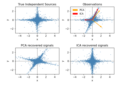
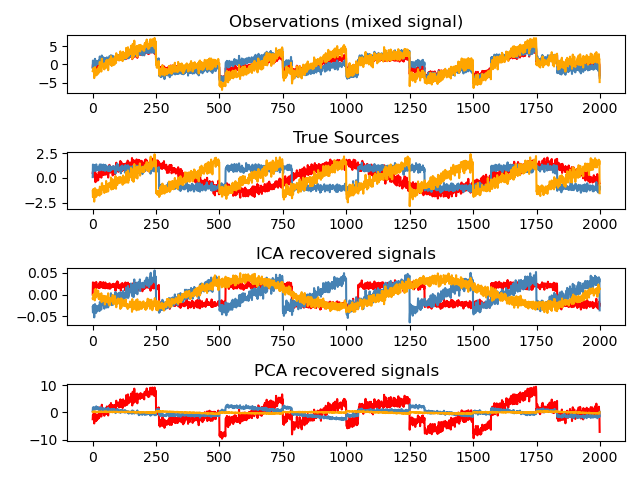
使用 FastICA 進行盲源分離#

從雜訊資料估計來源的範例。

獨立成分分析 (ICA)用於根據雜訊測量估計來源。想像一下 3 種樂器同時演奏，以及 3 個麥克風錄製混合訊號。ICA 用於還原來源，即每種樂器演奏的內容。重要的是，PCA 無法還原我們的 樂器，因為相關訊號反映非高斯過程。

# Authors: The scikit-learn developers
# SPDX-License-Identifier: BSD-3-Clause

產生範例資料#

import numpy as np
from scipy import signal

np.random.seed(0)
n_samples = 2000
time = np.linspace(0, 8, n_samples)

s1 = np.sin(2 * time)  # Signal 1 : sinusoidal signal
s2 = np.sign(np.sin(3 * time))  # Signal 2 : square signal
s3 = signal.sawtooth(2 * np.pi * time)  # Signal 3: saw tooth signal

S = np.c_[s1, s2, s3]
S += 0.2 * np.random.normal(size=S.shape)  # Add noise

S /= S.std(axis=0)  # Standardize data
# Mix data
A = np.array([[1, 1, 1], [0.5, 2, 1.0], [1.5, 1.0, 2.0]])  # Mixing matrix
X = np.dot(S, A.T)  # Generate observations

擬合 ICA 和 PCA 模型#

from sklearn.decomposition import PCA, FastICA

# Compute ICA
ica = FastICA(n_components=3, whiten="arbitrary-variance")
S_ = ica.fit_transform(X)  # Reconstruct signals
A_ = ica.mixing_  # Get estimated mixing matrix

# We can `prove` that the ICA model applies by reverting the unmixing.
assert np.allclose(X, np.dot(S_, A_.T) + ica.mean_)

# For comparison, compute PCA
pca = PCA(n_components=3)
H = pca.fit_transform(X)  # Reconstruct signals based on orthogonal components

繪製結果#

import matplotlib.pyplot as plt

plt.figure()

models = [X, S, S_, H]
names = [
    "Observations (mixed signal)",
    "True Sources",
    "ICA recovered signals",
    "PCA recovered signals",
]
colors = ["red", "steelblue", "orange"]

for ii, (model, name) in enumerate(zip(models, names), 1):
    plt.subplot(4, 1, ii)
    plt.title(name)
    for sig, color in zip(model.T, colors):
        plt.plot(sig, color=color)

plt.tight_layout()
plt.show()