多項式和樣條插值#

此範例示範如何使用嶺迴歸以最高 degree 的多項式來逼近函數。我們展示了兩種不同的方法，給定 n_samples 個 1 維點 x_i

PolynomialFeatures 會產生所有最高至 degree 的單項式。這給我們所謂的范德蒙矩陣，其具有 n_samples 列和 degree + 1 行
```
[[1, x_0, x_0 ** 2, x_0 ** 3, ..., x_0 ** degree],
 [1, x_1, x_1 ** 2, x_1 ** 3, ..., x_1 ** degree],
 ...]
```
直觀上，此矩陣可以解釋為偽特徵矩陣（點被提升到某個冪）。該矩陣類似於（但不同於）由多項式核心誘導的矩陣。
SplineTransformer 會產生 B 樣條基底函數。B 樣條的基底函數是 degree 次的分段多項式函數，僅在 degree+1 個連續節點之間非零。給定 n_knots 個節點數，這會產生一個 n_samples 列和 n_knots + degree - 1 行的矩陣
```
[[basis_1(x_0), basis_2(x_0), ...],
 [basis_1(x_1), basis_2(x_1), ...],
 ...]
```

此範例顯示這兩個轉換器非常適合使用線性模型對非線性效應建模，使用管道添加非線性特徵。核心方法擴展了這個概念，並且可以誘導非常高（甚至無限）維度的特徵空間。

# Authors: The scikit-learn developers
# SPDX-License-Identifier: BSD-3-Clause

import matplotlib.pyplot as plt
import numpy as np

from sklearn.linear_model import Ridge
from sklearn.pipeline import make_pipeline
from sklearn.preprocessing import PolynomialFeatures, SplineTransformer

我們先定義一個我們要逼近的函數，並準備繪製它。

def f(x):
    """Function to be approximated by polynomial interpolation."""
    return x * np.sin(x)


# whole range we want to plot
x_plot = np.linspace(-1, 11, 100)

為了讓它更有趣，我們只給一小部分點進行訓練。

x_train = np.linspace(0, 10, 100)
rng = np.random.RandomState(0)
x_train = np.sort(rng.choice(x_train, size=20, replace=False))
y_train = f(x_train)

# create 2D-array versions of these arrays to feed to transformers
X_train = x_train[:, np.newaxis]
X_plot = x_plot[:, np.newaxis]

現在我們準備好建立多項式特徵和樣條，在訓練點上進行擬合，並顯示它們的插值效果。

# plot function
lw = 2
fig, ax = plt.subplots()
ax.set_prop_cycle(
    color=["black", "teal", "yellowgreen", "gold", "darkorange", "tomato"]
)
ax.plot(x_plot, f(x_plot), linewidth=lw, label="ground truth")

# plot training points
ax.scatter(x_train, y_train, label="training points")

# polynomial features
for degree in [3, 4, 5]:
    model = make_pipeline(PolynomialFeatures(degree), Ridge(alpha=1e-3))
    model.fit(X_train, y_train)
    y_plot = model.predict(X_plot)
    ax.plot(x_plot, y_plot, label=f"degree {degree}")

# B-spline with 4 + 3 - 1 = 6 basis functions
model = make_pipeline(SplineTransformer(n_knots=4, degree=3), Ridge(alpha=1e-3))
model.fit(X_train, y_train)

y_plot = model.predict(X_plot)
ax.plot(x_plot, y_plot, label="B-spline")
ax.legend(loc="lower center")
ax.set_ylim(-20, 10)
plt.show()

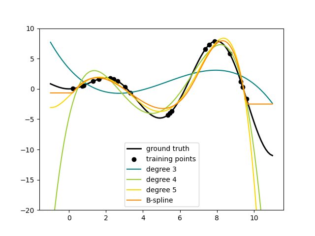
這清楚地表明，較高次數的多項式可以更好地擬合資料。但同時，太高的冪可能會顯示出不希望出現的振盪行為，並且對於超出擬合資料範圍的推斷特別危險。這是 B 樣條的優點。它們通常可以像多項式一樣擬合資料，並顯示出非常好的平滑行為。它們還有很好的選項可以控制推斷，預設為以常數繼續。請注意，在大多數情況下，您寧願增加節點數，但保持 degree=3。

為了更深入了解產生的特徵基底，我們分別繪製了兩個轉換器的所有列。

fig, axes = plt.subplots(ncols=2, figsize=(16, 5))
pft = PolynomialFeatures(degree=3).fit(X_train)
axes[0].plot(x_plot, pft.transform(X_plot))
axes[0].legend(axes[0].lines, [f"degree {n}" for n in range(4)])
axes[0].set_title("PolynomialFeatures")

splt = SplineTransformer(n_knots=4, degree=3).fit(X_train)
axes[1].plot(x_plot, splt.transform(X_plot))
axes[1].legend(axes[1].lines, [f"spline {n}" for n in range(6)])
axes[1].set_title("SplineTransformer")

# plot knots of spline
knots = splt.bsplines_[0].t
axes[1].vlines(knots[3:-3], ymin=0, ymax=0.8, linestyles="dashed")
plt.show()

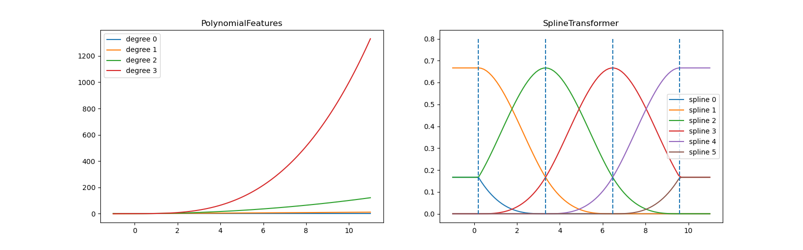
在左側的圖中，我們辨識出對應於從 x**0 到 x**3 的簡單單項式的直線。在右圖中，我們看到 degree=3 的六個 B 樣條基底函數，以及在 fit 期間選擇的四個節點位置。請注意，在擬合區間的左側和右側分別有 degree 個額外的節點。這些是為了技術原因而存在的，因此我們不顯示它們。每個基底函數都有局部支援，並且在擬合範圍之外以常數繼續。這種推斷行為可以透過參數 extrapolation 來變更。

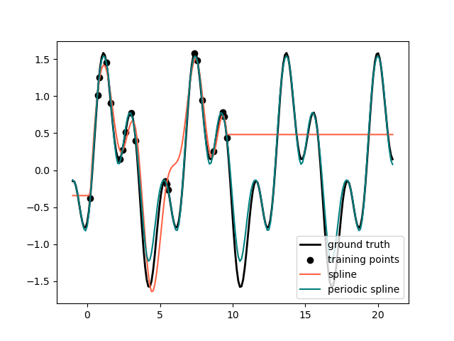
週期性樣條#

在先前的範例中，我們看到了多項式和樣條在訓練觀測範圍之外進行推斷的限制。在某些設定中，例如具有季節性效應的情況，我們預期基礎訊號會週期性地持續。此類效應可以使用週期性樣條來建模，該樣條在第一個和最後一個節點處具有相等的功能值和相等的導數。在以下情況下，我們將展示在給定週期性的額外資訊下，週期性樣條如何在訓練資料範圍內外提供更好的擬合。樣條週期是第一個和最後一個節點之間的距離，我們手動指定它。

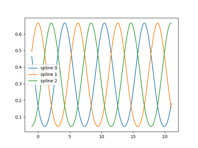
週期性樣條也可用於自然週期性特徵（例如一年中的某一天），因為邊界節點的平滑度可防止轉換值發生跳躍（例如，從 12 月 31 日到 1 月 1 日）。對於這種自然週期性特徵，或更一般地對於週期已知的特徵，建議透過手動設定節點將此資訊明確傳遞給 SplineTransformer。

def g(x):
    """Function to be approximated by periodic spline interpolation."""
    return np.sin(x) - 0.7 * np.cos(x * 3)


y_train = g(x_train)

# Extend the test data into the future:
x_plot_ext = np.linspace(-1, 21, 200)
X_plot_ext = x_plot_ext[:, np.newaxis]

lw = 2
fig, ax = plt.subplots()
ax.set_prop_cycle(color=["black", "tomato", "teal"])
ax.plot(x_plot_ext, g(x_plot_ext), linewidth=lw, label="ground truth")
ax.scatter(x_train, y_train, label="training points")

for transformer, label in [
    (SplineTransformer(degree=3, n_knots=10), "spline"),
    (
        SplineTransformer(
            degree=3,
            knots=np.linspace(0, 2 * np.pi, 10)[:, None],
            extrapolation="periodic",
        ),
        "periodic spline",
    ),
]:
    model = make_pipeline(transformer, Ridge(alpha=1e-3))
    model.fit(X_train, y_train)
    y_plot_ext = model.predict(X_plot_ext)
    ax.plot(x_plot_ext, y_plot_ext, label=label)

ax.legend()
fig.show()

fig, ax = plt.subplots()
knots = np.linspace(0, 2 * np.pi, 4)
splt = SplineTransformer(knots=knots[:, None], degree=3, extrapolation="periodic").fit(
    X_train
)
ax.plot(x_plot_ext, splt.transform(X_plot_ext))
ax.legend(ax.lines, [f"spline {n}" for n in range(3)])
plt.show()