注意
前往末尾下載完整範例程式碼。或透過 JupyterLite 或 Binder 在您的瀏覽器中執行此範例
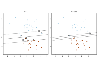
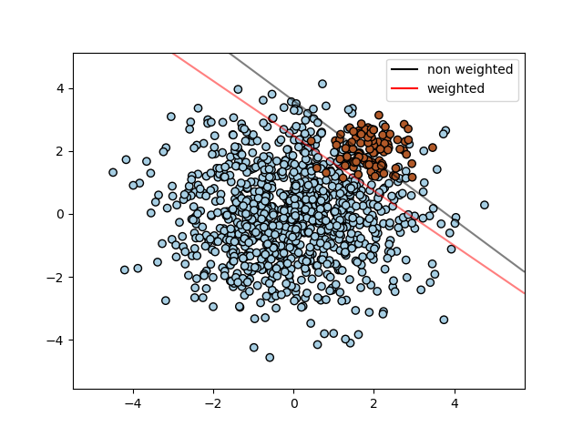
SVM:不平衡類別的分離超平面#
為不平衡的類別尋找使用 SVC 的最佳分離超平面。
我們首先找到具有普通 SVC 的分離平面,然後繪製(虛線)具有自動校正不平衡類別的分離超平面。
注意
此範例也可以透過將 SVC(kernel="linear") 替換為 SGDClassifier(loss="hinge") 來運作。將 SGDClassifier 的 loss 參數設定為等於 hinge 將會產生像帶有線性核的 SVC 的行為。
例如,嘗試使用 SGDClassifier(loss="hinge") 而不是 SVC
clf = SGDClassifier(n_iter=100, alpha=0.01)
# Authors: The scikit-learn developers
# SPDX-License-Identifier: BSD-3-Clause

import matplotlib.lines as mlines
import matplotlib.pyplot as plt

from sklearn import svm
from sklearn.datasets import make_blobs
from sklearn.inspection import DecisionBoundaryDisplay

# we create two clusters of random points
n_samples_1 = 1000
n_samples_2 = 100
centers = [[0.0, 0.0], [2.0, 2.0]]
clusters_std = [1.5, 0.5]
X, y = make_blobs(
    n_samples=[n_samples_1, n_samples_2],
    centers=centers,
    cluster_std=clusters_std,
    random_state=0,
    shuffle=False,
)

# fit the model and get the separating hyperplane
clf = svm.SVC(kernel="linear", C=1.0)
clf.fit(X, y)

# fit the model and get the separating hyperplane using weighted classes
wclf = svm.SVC(kernel="linear", class_weight={1: 10})
wclf.fit(X, y)

# plot the samples
plt.scatter(X[:, 0], X[:, 1], c=y, cmap=plt.cm.Paired, edgecolors="k")

# plot the decision functions for both classifiers
ax = plt.gca()
disp = DecisionBoundaryDisplay.from_estimator(
    clf,
    X,
    plot_method="contour",
    colors="k",
    levels=[0],
    alpha=0.5,
    linestyles=["-"],
    ax=ax,
)

# plot decision boundary and margins for weighted classes
wdisp = DecisionBoundaryDisplay.from_estimator(
    wclf,
    X,
    plot_method="contour",
    colors="r",
    levels=[0],
    alpha=0.5,
    linestyles=["-"],
    ax=ax,
)

plt.legend(
    [
        mlines.Line2D([], [], color="k", label="non weighted"),
        mlines.Line2D([], [], color="r", label="weighted"),
    ],
    ["non weighted", "weighted"],
    loc="upper right",
)
plt.show()
腳本的總執行時間: (0 分鐘 0.167 秒)
相關範例