注意
前往結尾以下載完整的範例程式碼。或者透過 JupyterLite 或 Binder 在您的瀏覽器中執行此範例
比較目標編碼器和其他編碼器#
TargetEncoder 使用目標的值來編碼每個類別特徵。在此範例中,我們將比較三種不同的方法來處理類別特徵:TargetEncoder、OrdinalEncoder、OneHotEncoder 和刪除類別。
注意
fit(X, y).transform(X) 不等於 fit_transform(X, y),因為編碼時在 fit_transform 中使用了交叉擬合方案。有關詳細資訊,請參閱使用者指南。
# Authors: The scikit-learn developers
# SPDX-License-Identifier: BSD-3-Clause
從 OpenML 載入資料#
首先,我們載入葡萄酒評論資料集,其中目標是評論者給出的分數
from sklearn.datasets import fetch_openml

wine_reviews = fetch_openml(data_id=42074, as_frame=True)

df = wine_reviews.frame
df.head()
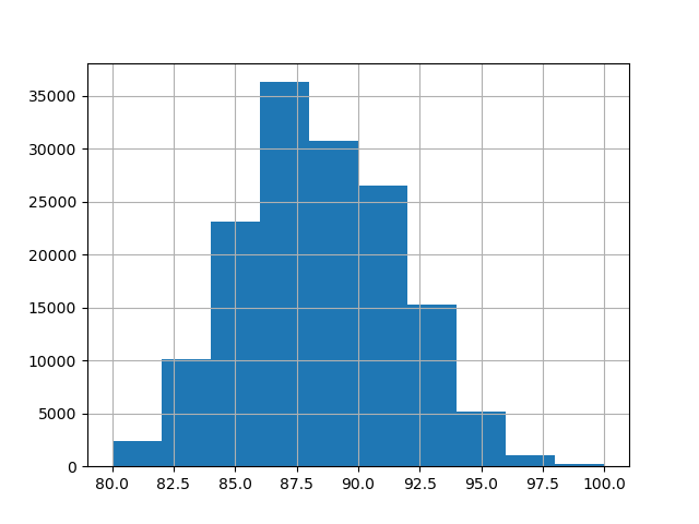
在此範例中,我們使用資料中數值和類別特徵的以下子集。目標是從 80 到 100 的連續值
numerical_features = ["price"]
categorical_features = [
    "country",
    "province",
    "region_1",
    "region_2",
    "variety",
    "winery",
]
target_name = "points"

X = df[numerical_features + categorical_features]
y = df[target_name]

_ = y.hist()
使用不同編碼器訓練和評估管線#
在本節中,我們將使用具有不同編碼策略的 HistGradientBoostingRegressor 評估管線。首先,我們列出將用於預處理類別特徵的編碼器
from sklearn.compose import ColumnTransformer
from sklearn.preprocessing import OneHotEncoder, OrdinalEncoder, TargetEncoder

categorical_preprocessors = [
    ("drop", "drop"),
    ("ordinal", OrdinalEncoder(handle_unknown="use_encoded_value", unknown_value=-1)),
    (
        "one_hot",
        OneHotEncoder(handle_unknown="ignore", max_categories=20, sparse_output=False),
    ),
    ("target", TargetEncoder(target_type="continuous")),
]
接下來,我們使用交叉驗證來評估模型並記錄結果
from sklearn.ensemble import HistGradientBoostingRegressor
from sklearn.model_selection import cross_validate
from sklearn.pipeline import make_pipeline

n_cv_folds = 3
max_iter = 20
results = []


def evaluate_model_and_store(name, pipe):
    result = cross_validate(
        pipe,
        X,
        y,
        scoring="neg_root_mean_squared_error",
        cv=n_cv_folds,
        return_train_score=True,
    )
    rmse_test_score = -result["test_score"]
    rmse_train_score = -result["train_score"]
    results.append(
        {
            "preprocessor": name,
            "rmse_test_mean": rmse_test_score.mean(),
            "rmse_test_std": rmse_train_score.std(),
            "rmse_train_mean": rmse_train_score.mean(),
            "rmse_train_std": rmse_train_score.std(),
        }
    )


for name, categorical_preprocessor in categorical_preprocessors:
    preprocessor = ColumnTransformer(
        [
            ("numerical", "passthrough", numerical_features),
            ("categorical", categorical_preprocessor, categorical_features),
        ]
    )
    pipe = make_pipeline(
        preprocessor, HistGradientBoostingRegressor(random_state=0, max_iter=max_iter)
    )
    evaluate_model_and_store(name, pipe)
原生類別特徵支援#
在本節中,我們建立並評估一個管線,該管線在 HistGradientBoostingRegressor 中使用原生類別特徵支援,該支援僅支援最多 255 個唯一類別。在我們的資料集中,大多數類別特徵具有超過 255 個唯一類別
n_unique_categories = df[categorical_features].nunique().sort_values(ascending=False)
n_unique_categories
winery      14810
region_1     1236
variety       632
province      455
country        48
region_2       18
dtype: int64
為了解決上述限制,我們將類別特徵分為低基數和高基數特徵。高基數特徵將進行目標編碼,而低基數特徵將使用梯度提升中的原生類別特徵。
high_cardinality_features = n_unique_categories[n_unique_categories > 255].index
low_cardinality_features = n_unique_categories[n_unique_categories <= 255].index
mixed_encoded_preprocessor = ColumnTransformer(
    [
        ("numerical", "passthrough", numerical_features),
        (
            "high_cardinality",
            TargetEncoder(target_type="continuous"),
            high_cardinality_features,
        ),
        (
            "low_cardinality",
            OrdinalEncoder(handle_unknown="use_encoded_value", unknown_value=-1),
            low_cardinality_features,
        ),
    ],
    verbose_feature_names_out=False,
)

# The output of the of the preprocessor must be set to pandas so the
# gradient boosting model can detect the low cardinality features.
mixed_encoded_preprocessor.set_output(transform="pandas")
mixed_pipe = make_pipeline(
    mixed_encoded_preprocessor,
    HistGradientBoostingRegressor(
        random_state=0, max_iter=max_iter, categorical_features=low_cardinality_features
    ),
)
mixed_pipe
最後,我們使用交叉驗證來評估管線並記錄結果
evaluate_model_and_store("mixed_target", mixed_pipe)
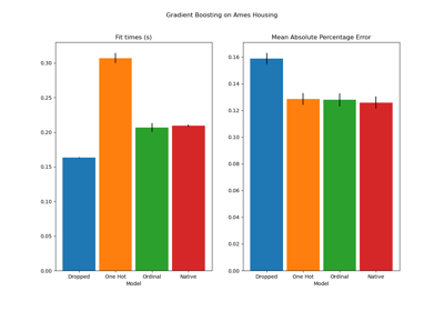
繪製結果#
在本節中,我們透過繪製測試和訓練分數來顯示結果
import matplotlib.pyplot as plt
import pandas as pd

results_df = (
    pd.DataFrame(results).set_index("preprocessor").sort_values("rmse_test_mean")
)

fig, (ax1, ax2) = plt.subplots(
    1, 2, figsize=(12, 8), sharey=True, constrained_layout=True
)
xticks = range(len(results_df))
name_to_color = dict(
    zip((r["preprocessor"] for r in results), ["C0", "C1", "C2", "C3", "C4"])
)

for subset, ax in zip(["test", "train"], [ax1, ax2]):
    mean, std = f"rmse_{subset}_mean", f"rmse_{subset}_std"
    data = results_df[[mean, std]].sort_values(mean)
    ax.bar(
        x=xticks,
        height=data[mean],
        yerr=data[std],
        width=0.9,
        color=[name_to_color[name] for name in data.index],
    )
    ax.set(
        title=f"RMSE ({subset.title()})",
        xlabel="Encoding Scheme",
        xticks=xticks,
        xticklabels=data.index,
    )
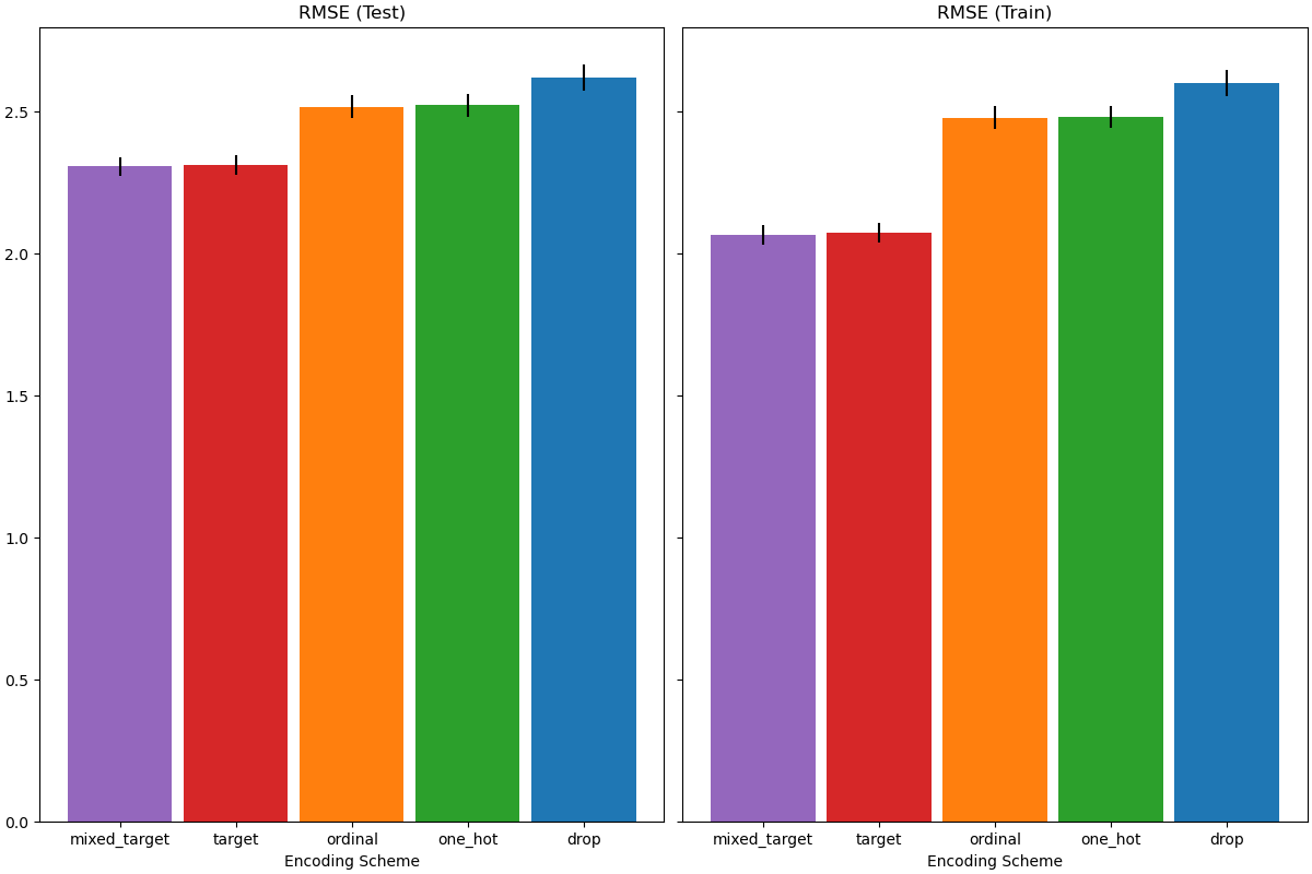
在評估測試集上的預測效能時,刪除類別的效能最差,而目標編碼器的效能最好。這可以解釋如下
刪除類別特徵會使管線的表達能力降低,並導致欠擬合;
由於基數高且為了減少訓練時間,單熱編碼方案使用
max_categories=20,這可防止特徵擴展過多,這可能會導致欠擬合。如果我們沒有設定
max_categories=20,那麼單熱編碼方案很可能會使管線過擬合,因為特徵的數量隨著與目標偶然相關的罕見類別出現次數而爆炸(僅在訓練集上);序數編碼對特徵施加了任意順序,然後
HistGradientBoostingRegressor將其視為數值。由於此模型將每個特徵的數值特徵分組為 256 個 bin,因此許多不相關的類別可以分組在一起,因此整體管線可能會欠擬合;當使用目標編碼器時,也會發生相同的分箱,但由於編碼值是通過與目標變數的邊際關聯統計排序的,因此
HistGradientBoostingRegressor使用的分箱是有意義的,並帶來了良好的結果:平滑目標編碼和分箱的組合可以作為一種良好的正規化策略來防止過擬合,同時又不會過度限制管線的表達能力。
腳本總執行時間: (0 分鐘 26.981 秒)
相關範例