注意
跳到結尾以下載完整的範例程式碼。或者透過 JupyterLite 或 Binder 在您的瀏覽器中執行此範例
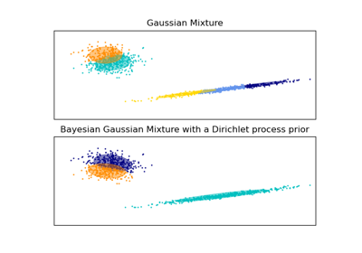
高斯混合模型選擇#
此範例示範如何使用資訊理論準則,使用高斯混合模型(GMM)進行模型選擇。模型選擇同時涉及共變異數類型和模型中的組件數量。
在此案例中,Akaike 資訊準則(AIC)和貝氏資訊準則(BIC)都提供了正確的結果,但我們僅示範後者,因為 BIC 更適合在候選集合中識別真實模型。與貝氏程序不同,此類推論是無先驗的。
# Authors: The scikit-learn developers
# SPDX-License-Identifier: BSD-3-Clause
資料產生#
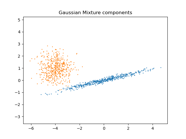
我們產生兩個組件(每個組件包含 n_samples),方法是隨機取樣由 numpy.random.randn 返回的標準常態分佈。一個組件保持球形,但已移動和重新縮放。另一個組件變形為具有更一般的共變異數矩陣。
import numpy as np

n_samples = 500
np.random.seed(0)
C = np.array([[0.0, -0.1], [1.7, 0.4]])
component_1 = np.dot(np.random.randn(n_samples, 2), C)  # general
component_2 = 0.7 * np.random.randn(n_samples, 2) + np.array([-4, 1])  # spherical

X = np.concatenate([component_1, component_2])
我們可以視覺化不同的組件
import matplotlib.pyplot as plt

plt.scatter(component_1[:, 0], component_1[:, 1], s=0.8)
plt.scatter(component_2[:, 0], component_2[:, 1], s=0.8)
plt.title("Gaussian Mixture components")
plt.axis("equal")
plt.show()
模型訓練和選擇#
我們將組件數量從 1 變更到 6,並變更要使用的共變異數參數類型
"full":每個組件都有其自己的通用共變異數矩陣。"tied":所有組件共用相同的通用共變異數矩陣。"diag":每個組件都有其自己的對角共變異數矩陣。"spherical":每個組件都有其自己的單個變異數。
我們為不同的模型評分,並保留最佳模型(最低的 BIC)。這是透過使用GridSearchCV和使用者定義的評分函數(返回負 BIC 分數)來完成,因為GridSearchCV旨在最大化分數(最大化負 BIC 等於最小化 BIC)。
最佳參數集和估計器分別儲存在 best_parameters_ 和 best_estimator_ 中。
from sklearn.mixture import GaussianMixture
from sklearn.model_selection import GridSearchCV


def gmm_bic_score(estimator, X):
    """Callable to pass to GridSearchCV that will use the BIC score."""
    # Make it negative since GridSearchCV expects a score to maximize
    return -estimator.bic(X)


param_grid = {
    "n_components": range(1, 7),
    "covariance_type": ["spherical", "tied", "diag", "full"],
}
grid_search = GridSearchCV(
    GaussianMixture(), param_grid=param_grid, scoring=gmm_bic_score
)
grid_search.fit(X)
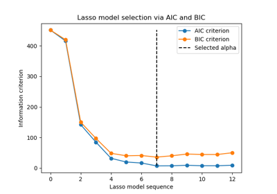
繪製 BIC 分數#
為了方便繪圖,我們可以從網格搜尋完成的交叉驗證結果建立 pandas.DataFrame。我們反轉 BIC 分數的符號,以顯示將其最小化的效果。
import pandas as pd

df = pd.DataFrame(grid_search.cv_results_)[
    ["param_n_components", "param_covariance_type", "mean_test_score"]
]
df["mean_test_score"] = -df["mean_test_score"]
df = df.rename(
    columns={
        "param_n_components": "Number of components",
        "param_covariance_type": "Type of covariance",
        "mean_test_score": "BIC score",
    }
)
df.sort_values(by="BIC score").head()
import seaborn as sns

sns.catplot(
    data=df,
    kind="bar",
    x="Number of components",
    y="BIC score",
    hue="Type of covariance",
)
plt.show()
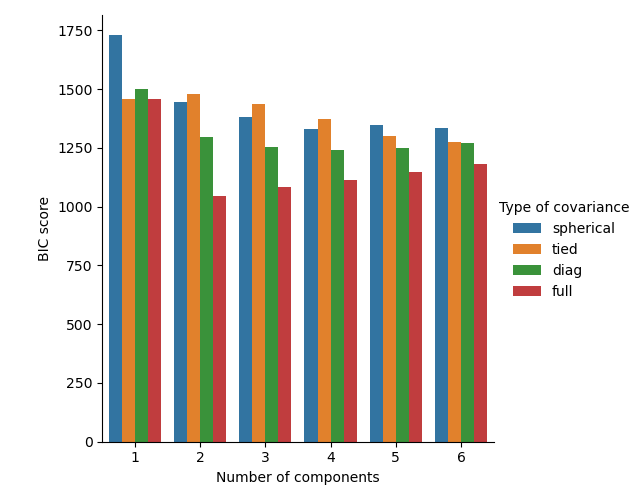
在目前案例中,具有 2 個組件和完整共變異數(對應於真實生成模型)的模型具有最低的 BIC 分數,因此由網格搜尋選取。
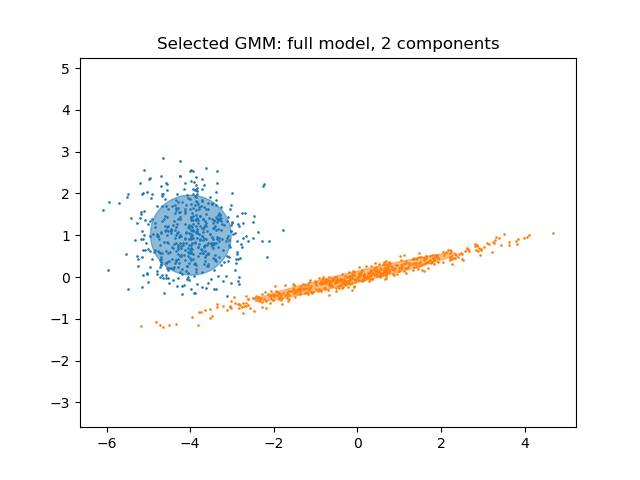
繪製最佳模型#
我們繪製一個橢圓以顯示選定模型的每個高斯組件。為此,需要找到由 covariances_ 屬性傳回的共變異數矩陣的特徵值。此類矩陣的形狀取決於 covariance_type
"full":(n_components,n_features,n_features)"tied":(n_features,n_features)"diag":(n_components,n_features)"spherical":(n_components,)
from matplotlib.patches import Ellipse
from scipy import linalg

color_iter = sns.color_palette("tab10", 2)[::-1]
Y_ = grid_search.predict(X)

fig, ax = plt.subplots()

for i, (mean, cov, color) in enumerate(
    zip(
        grid_search.best_estimator_.means_,
        grid_search.best_estimator_.covariances_,
        color_iter,
    )
):
    v, w = linalg.eigh(cov)
    if not np.any(Y_ == i):
        continue
    plt.scatter(X[Y_ == i, 0], X[Y_ == i, 1], 0.8, color=color)

    angle = np.arctan2(w[0][1], w[0][0])
    angle = 180.0 * angle / np.pi  # convert to degrees
    v = 2.0 * np.sqrt(2.0) * np.sqrt(v)
    ellipse = Ellipse(mean, v[0], v[1], angle=180.0 + angle, color=color)
    ellipse.set_clip_box(fig.bbox)
    ellipse.set_alpha(0.5)
    ax.add_artist(ellipse)

plt.title(
    f"Selected GMM: {grid_search.best_params_['covariance_type']} model, "
    f"{grid_search.best_params_['n_components']} components"
)
plt.axis("equal")
plt.show()
腳本總執行時間:(0 分鐘 1.388 秒)
相關範例