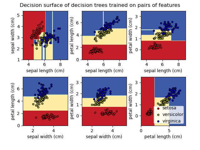
繪製在鳶尾花資料集上訓練的決策樹的決策面#

繪製在鳶尾花資料集的特徵對上訓練的決策樹的決策面。

請參閱決策樹以取得有關估計器的更多資訊。

對於每對鳶尾花特徵，決策樹會學習由從訓練樣本推斷出的簡單閾值規則組合而成的決策邊界。

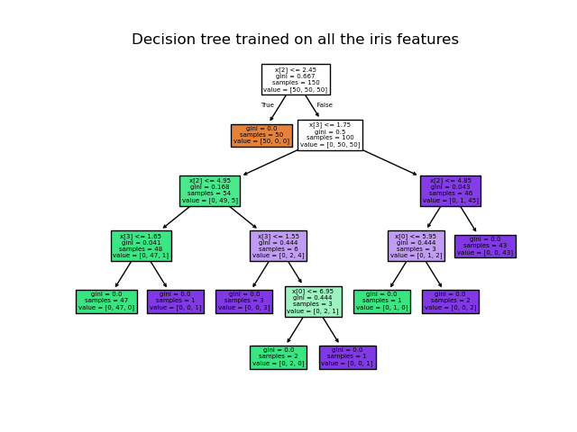
我們還展示了基於所有特徵建立的模型的樹狀結構。

# Authors: The scikit-learn developers
# SPDX-License-Identifier: BSD-3-Clause

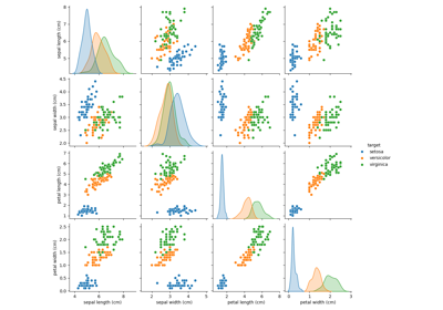
首先載入 scikit-learn 隨附的鳶尾花資料集副本

from sklearn.datasets import load_iris

iris = load_iris()

顯示在所有特徵對上訓練的樹的決策函數。

import matplotlib.pyplot as plt
import numpy as np

from sklearn.datasets import load_iris
from sklearn.inspection import DecisionBoundaryDisplay
from sklearn.tree import DecisionTreeClassifier

# Parameters
n_classes = 3
plot_colors = "ryb"
plot_step = 0.02


for pairidx, pair in enumerate([[0, 1], [0, 2], [0, 3], [1, 2], [1, 3], [2, 3]]):
    # We only take the two corresponding features
    X = iris.data[:, pair]
    y = iris.target

    # Train
    clf = DecisionTreeClassifier().fit(X, y)

    # Plot the decision boundary
    ax = plt.subplot(2, 3, pairidx + 1)
    plt.tight_layout(h_pad=0.5, w_pad=0.5, pad=2.5)
    DecisionBoundaryDisplay.from_estimator(
        clf,
        X,
        cmap=plt.cm.RdYlBu,
        response_method="predict",
        ax=ax,
        xlabel=iris.feature_names[pair[0]],
        ylabel=iris.feature_names[pair[1]],
    )

    # Plot the training points
    for i, color in zip(range(n_classes), plot_colors):
        idx = np.where(y == i)
        plt.scatter(
            X[idx, 0],
            X[idx, 1],
            c=color,
            label=iris.target_names[i],
            edgecolor="black",
            s=15,
        )

plt.suptitle("Decision surface of decision trees trained on pairs of features")
plt.legend(loc="lower right", borderpad=0, handletextpad=0)
_ = plt.axis("tight")

Decision surface of decision trees trained on pairs of features

顯示在所有特徵一起訓練的單個決策樹的結構。

from sklearn.tree import plot_tree

plt.figure()
clf = DecisionTreeClassifier().fit(iris.data, iris.target)
plot_tree(clf, filled=True)
plt.title("Decision tree trained on all the iris features")
plt.show()